RAG Blueprint tutorial
Many of our users use Vespa to power large scale RAG Applications.
This blueprint aims to exemplify many of the best practices we have learned while supporting these users.
While many RAG tutorials exist, this blueprint provides a customizable template that:
- Can (auto)scale with your data size and/or query load.
- Is fast and production grade.
- Enables you to build RAG applications with state-of-the-art quality.
This tutorial will show how we can develop a high-quality RAG application with an evaluation-driven mindset, while being a resource you can revisit for making informed choices for your own use case.
We will guide you through the following steps:
- Installing dependencies
- Cloning the RAG Blueprint
- Inspecting the RAG Blueprint
- Deploying to Vespa Cloud
- Our use case
- Data modeling
- Structuring your Vespa application
- Configuring match-phase (retrieval)
- First-phase ranking
- Second-phase ranking
- (Optional) Global-phase reranking
All the accompanying code can be found in our sample app repo, but we will also clone the repo and run the code in this notebook.
Some of the python scripts from the sample app will be adapted and shown inline in this notebook instead of running them separately.
Each step will contain reasoning behind the choices and design of the blueprint, as well as pointers for customizing to your own application.
This is not a 'Deploy RAG in 5 minutes' tutorial (although you can technically do that by just running the notebook). This focus is more about providing you with the insights and tools for you to apply it to your own use case. Therefore we suggest taking your time to look at the code in the sample app, and run the described steps."
![]()
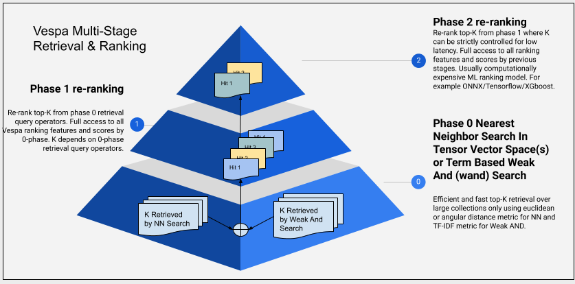
Here is an overview of the retrieval and ranking pipeline we will build in this tutorial:

Installing dependencies
!pip3 install pyvespa>=0.58.0 vespacli scikit-learn lightgbm pandas
zsh:1: 0.58.0 not found
Cloning the RAG Blueprint
Although you could define all components of the application with python code only from pyvespa, this would go against our advise on or the Advanced Configuration notebook for a guide if you want to do that.
Here, we will use pyvespa to deploy an application package from the existing files. Let us start by cloning the RAG Blueprint application from the Vespa sample-apps repository.
# Clone the RAG Blueprint sample application
!git clone --depth 1 --filter=blob:none --sparse https://github.com/vespa-engine/sample-apps.git src && cd src && git sparse-checkout set rag-blueprint
Cloning into 'src'...
remote: Enumerating objects: 640, done.
remote: Counting objects: 100% (640/640), done.
remote: Compressing objects: 100% (350/350), done.
remote: Total 640 (delta 7), reused 557 (delta 5), pack-reused 0 (from 0)
Receiving objects: 100% (640/640), 62.63 KiB | 1.01 MiB/s, done.
Resolving deltas: 100% (7/7), done.
remote: Enumerating objects: 15, done.
remote: Counting objects: 100% (15/15), done.
remote: Compressing objects: 100% (13/13), done.
remote: Total 15 (delta 2), reused 8 (delta 2), pack-reused 0 (from 0)
Receiving objects: 100% (15/15), 92.91 KiB | 318.00 KiB/s, done.
Resolving deltas: 100% (2/2), done.
Updating files: 100% (15/15), done.
remote: Enumerating objects: 37, done.
remote: Counting objects: 100% (37/37), done.
remote: Compressing objects: 100% (30/30), done.
remote: Total 37 (delta 8), reused 21 (delta 6), pack-reused 0 (from 0)
Receiving objects: 100% (37/37), 111.45 KiB | 401.00 KiB/s, done.
Resolving deltas: 100% (8/8), done.
Updating files: 100% (37/37), done.
Inspecting the RAG Blueprint
First, let's examine the structure of the RAG Blueprint application we just cloned:
from pathlib import Path


def tree(
    root: str | Path = ".", *, show_hidden: bool = False, max_depth: int | None = None
) -> str:
    """
    Return a Unix‐style 'tree' listing for *root*.

    Parameters
    ----------
    root : str | Path
        Directory to walk (default: ".")
    show_hidden : bool
        Include dotfiles and dot-dirs? (default: False)
    max_depth : int | None
        Limit recursion depth; None = no limit.

    Returns
    -------
    str
        A newline-joined string identical to `tree` output.
    """
    root_path = Path(root).resolve()
    lines = [root_path.as_posix()]

    def _walk(current: Path, prefix: str = "", depth: int = 0) -> None:
        if max_depth is not None and depth >= max_depth:
            return

        entries = sorted(
            (e for e in current.iterdir() if show_hidden or not e.name.startswith(".")),
            key=lambda p: (not p.is_dir(), p.name.lower()),
        )
        last = len(entries) - 1

        for idx, entry in enumerate(entries):
            connector = "└── " if idx == last else "├── "
            lines.append(f"{prefix}{connector}{entry.name}")
            if entry.is_dir():
                extension = "    " if idx == last else "│   "
                _walk(entry, prefix + extension, depth + 1)

    _walk(root_path)
    return "\n".join(lines)
# Let's explore the RAG Blueprint application structure
print(tree("src/rag-blueprint"))
/Users/thomas/Repos/pyvespa/docs/sphinx/source/examples/src/rag-blueprint
├── app
│   ├── models
│   │   └── lightgbm_model.json
│   ├── schemas
│   │   ├── doc
│   │   │   ├── base-features.profile
│   │   │   ├── collect-second-phase.profile
│   │   │   ├── collect-training-data.profile
│   │   │   ├── learned-linear.profile
│   │   │   ├── match-only.profile
│   │   │   └── second-with-gbdt.profile
│   │   └── doc.sd
│   ├── search
│   │   └── query-profiles
│   │       ├── deepresearch-with-gbdt.xml
│   │       ├── deepresearch.xml
│   │       ├── hybrid-with-gbdt.xml
│   │       ├── hybrid.xml
│   │       ├── rag-with-gbdt.xml
│   │       └── rag.xml
│   └── services.xml
├── dataset
│   └── docs.jsonl
├── eval
│   ├── output
│   │   ├── Vespa-training-data_match_first_phase_20250623_133241.csv
│   │   ├── Vespa-training-data_match_first_phase_20250623_133241_logreg_coefficients.txt
│   │   ├── Vespa-training-data_match_rank_second_phase_20250623_135819.csv
│   │   └── Vespa-training-data_match_rank_second_phase_20250623_135819_feature_importance.csv
│   ├── collect_pyvespa.py
│   ├── evaluate_match_phase.py
│   ├── evaluate_ranking.py
│   ├── pyproject.toml
│   ├── README.md
│   ├── resp.json
│   ├── train_lightgbm.py
│   └── train_logistic_regression.py
├── queries
│   ├── queries.json
│   └── test_queries.json
├── deploy-locally.md
├── generation.md
├── query-profiles.md
├── README.md
└── relevance.md
We can see that the RAG Blueprint includes a complete application package with:
schemas/doc.sd- The document schema with chunking and embeddingsschemas/doc/*.profile- Ranking profiles for collecting training data, first-phase ranking, and second-phase rankingservices.xml- Services configuration with embedder and LLM integrationsearch/query-profiles/*.xml- Pre-configured query profiles for different use casesmodels/- Pre-trained ranking models
Deploying to Vespa Cloud
from vespa.deployment import VespaCloud
from vespa.application import Vespa
from pathlib import Path
import os
import json
VESPA_TENANT_NAME = "vespa-team" # Replace with your tenant name
Here, set your desired application name. (Will be created in later steps)
Note that you can not have hyphen - or underscore _ in the application name.
VESPA_APPLICATION_NAME = "rag-blueprint"  # No hyphens or underscores allowed
VESPA_SCHEMA_NAME = "doc"  # RAG Blueprint uses 'doc' schema
repo_root = Path("src/rag-blueprint")
application_root = repo_root / "app"
Note, you could also enable a token endpoint, for easier connection after deployment, see Authenticating to Vespa Cloud for details. We will stick to the default MTLS key/cert authentication for this notebook.
Adding secret to Vespa Cloud Secret Store
In order to use the LLM integration, you need to add your OpenAI API key to the Vespa Cloud Secret Store.
Then, we can reference this secret in our services.xml file, so that Vespa can use it to access the OpenAI API.
Below we have added a vault called sample-apps and a secret named openai-dev that contains the OpenAI API key.
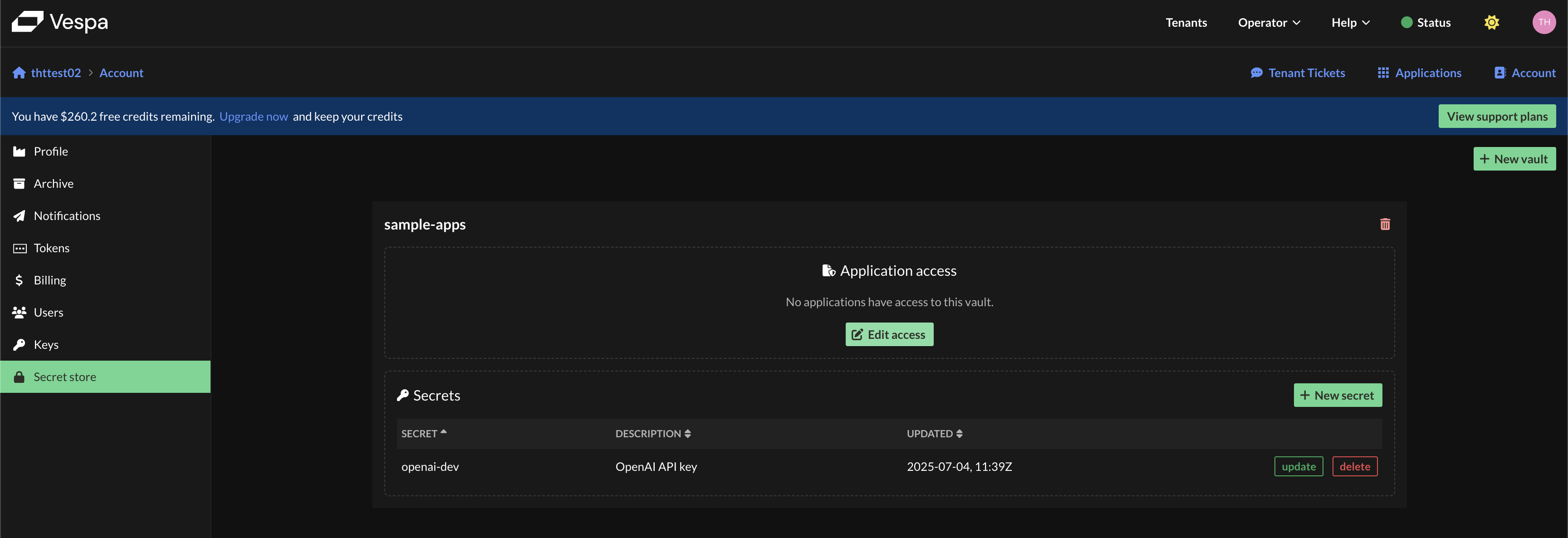
Make sure that the vault and secret names match the ones in the services.xml file.
        <secrets>
            <openai-api-key vault="sample-apps" name="openai-dev" />
        </secrets>
Let us first take a look at the original services.xml file, which contains the configuration for the Vespa application services, including the LLM integration and embedder.
!!! note It is also possible to define the services.xml-configuration in python code, see Advanced Configuration.
from IPython.display import display, Markdown


def display_md(text: str, tag: str = "txt"):
    text = text.rstrip()
    md = f"""```{tag}
{text}
```"""
    display(Markdown(md))


services_content = (application_root / "services.xml").read_text()
display_md(services_content, "xml")
<?xml version="1.0" encoding="utf-8"?>
<!-- Copyright Vespa.ai. Licensed under the terms of the Apache 2.0 license. See LICENSE in the
project root. -->
<services version="1.0" xmlns:deploy="vespa" xmlns:preprocess="properties"
    minimum-required-vespa-version="8.519.55">

    <container id="default" version="1.0">
        <document-processing />
        <document-api />
        <secrets>
            <openai-api-key vault="sample-apps" name="openai-dev" />
        </secrets>
        <!-- Setup the client to OpenAI -->
        <component id="openai" class="ai.vespa.llm.clients.OpenAI">
            <config name="ai.vespa.llm.clients.llm-client">
                <apiKeySecretName>openai-api-key</apiKeySecretName>
            </config>
        </component>

        <component id="nomicmb" type="hugging-face-embedder">
            <transformer-model
                url="https://data.vespa-cloud.com/onnx_models/nomic-ai-modernbert-embed-base/model.onnx" />
            <transformer-token-type-ids />
            <tokenizer-model
                url="https://data.vespa-cloud.com/onnx_models/nomic-ai-modernbert-embed-base/tokenizer.json" />
            <transformer-output>token_embeddings</transformer-output>
            <max-tokens>8192</max-tokens>
            <prepend>
                <query>search_query:</query>
                <document>search_document:</document>
            </prepend>
        </component>
        <search>
            <chain id="openai" inherits="vespa">
                <searcher id="ai.vespa.search.llm.RAGSearcher">
                    <config name="ai.vespa.search.llm.llm-searcher">
                        <providerId>openai</providerId>
                    </config>
                </searcher>
            </chain>
        </search>
        <nodes>
            <node hostalias="node1" />
        </nodes>
    </container>

    <!-- See https://docs.vespa.ai/en/reference/services-content.html -->
    <content id="content" version="1.0">
        <min-redundancy>2</min-redundancy>
        <documents>
            <document type="doc" mode="index" />
        </documents>
        <nodes>
            <node hostalias="node1" distribution-key="0" />
        </nodes>
    </content>

</services>
Deploy the application to Vespa Cloud
Now let's deploy the RAG Blueprint application to Vespa Cloud:
# This is only needed for CI.
VESPA_TEAM_API_KEY = os.getenv("VESPA_TEAM_API_KEY", None)
vespa_cloud = VespaCloud(
    tenant=VESPA_TENANT_NAME,
    application=VESPA_APPLICATION_NAME,
    key_content=VESPA_TEAM_API_KEY,
    application_root=application_root,
)
Setting application...
Running: vespa config set application vespa-team.rag-blueprint.default
Setting target cloud...
Running: vespa config set target cloud

Api-key found for control plane access. Using api-key.
Now, we will deploy the application to Vespa Cloud. This will take a few minutes, so feel free to skip ahead to the next section while waiting for the deployment to complete.
# Deploy the application
app: Vespa = vespa_cloud.deploy(disk_folder=application_root)
Deployment started in run 85 of dev-aws-us-east-1c for vespa-team.rag-blueprint. This may take a few minutes the first time.
INFO    [09:40:36]  Deploying platform version 8.586.25 and application dev build 85 for dev-aws-us-east-1c of default ...
INFO    [09:40:36]  Using CA signed certificate version 5
INFO    [09:40:43]  Session 379704 for tenant 'vespa-team' prepared and activated.
INFO    [09:40:43]  ######## Details for all nodes ########
INFO    [09:40:43]  h125699b.dev.us-east-1c.aws.vespa-cloud.net: expected to be UP
INFO    [09:40:43]  --- platform vespa/cloud-tenant-rhel8:8.586.25
INFO    [09:40:43]  --- storagenode on port 19102 has config generation 379704, wanted is 379704
INFO    [09:40:43]  --- searchnode on port 19107 has config generation 379704, wanted is 379704
INFO    [09:40:43]  --- distributor on port 19111 has config generation 379699, wanted is 379704
INFO    [09:40:43]  --- metricsproxy-container on port 19092 has config generation 379704, wanted is 379704
INFO    [09:40:43]  h125755a.dev.us-east-1c.aws.vespa-cloud.net: expected to be UP
INFO    [09:40:43]  --- platform vespa/cloud-tenant-rhel8:8.586.25
INFO    [09:40:43]  --- container on port 4080 has config generation 379699, wanted is 379704
INFO    [09:40:43]  --- metricsproxy-container on port 19092 has config generation 379704, wanted is 379704
INFO    [09:40:43]  h97530b.dev.us-east-1c.aws.vespa-cloud.net: expected to be UP
INFO    [09:40:43]  --- platform vespa/cloud-tenant-rhel8:8.586.25
INFO    [09:40:43]  --- logserver-container on port 4080 has config generation 379704, wanted is 379704
INFO    [09:40:43]  --- metricsproxy-container on port 19092 has config generation 379704, wanted is 379704
INFO    [09:40:43]  h119190c.dev.us-east-1c.aws.vespa-cloud.net: expected to be UP
INFO    [09:40:43]  --- platform vespa/cloud-tenant-rhel8:8.586.25
INFO    [09:40:43]  --- container-clustercontroller on port 19050 has config generation 379699, wanted is 379704
INFO    [09:40:43]  --- metricsproxy-container on port 19092 has config generation 379699, wanted is 379704
INFO    [09:40:51]  Found endpoints:
INFO    [09:40:51]  - dev.aws-us-east-1c
INFO    [09:40:51]   |-- https://fe5fe13c.fe19121d.z.vespa-app.cloud/ (cluster 'default')
INFO    [09:40:51]  Deployment of new application revision complete!
Only region: aws-us-east-1c available in dev environment.
Found mtls endpoint for default
URL: https://fe5fe13c.fe19121d.z.vespa-app.cloud/
Application is up!
Feed Sample Data
The RAG Blueprint comes with sample data. Let's download and feed it to test our deployment:
doc_file = repo_root / "dataset" / "docs.jsonl"
with open(doc_file, "r") as f:
    docs = [json.loads(line) for line in f.readlines()]
docs[:2]
[{'put': 'id:doc:doc::1',
  'fields': {'created_timestamp': 1675209600,
   'modified_timestamp': 1675296000,
   'text': '# SynapseCore Module: Custom Attention Implementation\n\n```python\nimport torch\nimport torch.nn as nn\nimport torch.nn.functional as F\n\nclass CustomAttention(nn.Module):\n    def __init__(self, hidden_dim):\n        super(CustomAttention, self).__init__()\n        self.hidden_dim = hidden_dim\n        self.query_layer = nn.Linear(hidden_dim, hidden_dim)\n        self.key_layer = nn.Linear(hidden_dim, hidden_dim)\n        self.value_layer = nn.Linear(hidden_dim, hidden_dim)\n        # More layers and logic here\n\n    def forward(self, query_input, key_input, value_input, mask=None):\n        # Q, K, V projections\n        Q = self.query_layer(query_input)\n        K = self.key_layer(key_input)\n        V = self.value_layer(value_input)\n\n        # Scaled Dot-Product Attention\n        attention_scores = torch.matmul(Q, K.transpose(-2, -1)) / (self.hidden_dim ** 0.5)\n        if mask is not None:\n            attention_scores = attention_scores.masked_fill(mask == 0, -1e9)\n        \n        attention_probs = F.softmax(attention_scores, dim=-1)\n        context_vector = torch.matmul(attention_probs, V)\n        return context_vector, attention_probs\n\n# Example Usage:\n# attention_module = CustomAttention(hidden_dim=512)\n# output, probs = attention_module(q_tensor, k_tensor, v_tensor)\n```\n\n## Design Notes:\n- Optimized for speed with batched operations.\n- Includes optional masking for variable sequence lengths.\n## <MORE_TEXT:HERE>',
   'favorite': True,
   'last_opened_timestamp': 1717308000,
   'open_count': 25,
   'title': 'custom_attention_impl.py.md',
   'id': '1'}},
 {'put': 'id:doc:doc::2',
  'fields': {'created_timestamp': 1709251200,
   'modified_timestamp': 1709254800,
   'text': "# YC Workshop Notes: Scaling B2B Sales (W25)\nDate: 2025-03-01\nSpeaker: [YC Partner Name]\n\n## Key Takeaways:\n1.  **ICP Definition is Crucial:** Don't try to sell to everyone. Narrow down your Ideal Customer Profile.\n    -   Characteristics: Industry, company size, pain points, decision-maker roles.\n2.  **Outbound Strategy:**\n    -   Personalized outreach > Mass emails.\n    -   Tools mentioned: Apollo.io, Outreach.io.\n    -   Metrics: Open rates, reply rates, meeting booked rates.\n3.  **Sales Process Stages:**\n    -   Prospecting -> Qualification -> Demo -> Proposal -> Negotiation -> Close.\n    -   Define clear entry/exit criteria for each stage.\n4.  **Value Proposition:** Clearly articulate how you solve the customer's pain and deliver ROI.\n5.  **Early Hires:** First sales hire should be a 'hunter-farmer' hybrid if possible, or a strong individual contributor.\n\n## Action Items for SynapseFlow:\n-   [ ] Refine ICP based on beta user feedback.\n-   [ ] Experiment with a small, targeted outbound campaign for 2 specific verticals.\n-   [ ] Draft initial sales playbook outline.\n## <MORE_TEXT:HERE>",
   'favorite': True,
   'last_opened_timestamp': 1717000000,
   'open_count': 12,
   'title': 'yc_b2b_sales_workshop_notes.md',
   'id': '2'}}]
vespa_feed = []
for doc in docs:
    vespa_doc = doc.copy()
    vespa_doc["id"] = doc["fields"]["id"]
    vespa_doc.pop("put")
    vespa_feed.append(vespa_doc)
vespa_feed[:2]
[{'fields': {'created_timestamp': 1675209600,
   'modified_timestamp': 1675296000,
   'text': '# SynapseCore Module: Custom Attention Implementation\n\n```python\nimport torch\nimport torch.nn as nn\nimport torch.nn.functional as F\n\nclass CustomAttention(nn.Module):\n    def __init__(self, hidden_dim):\n        super(CustomAttention, self).__init__()\n        self.hidden_dim = hidden_dim\n        self.query_layer = nn.Linear(hidden_dim, hidden_dim)\n        self.key_layer = nn.Linear(hidden_dim, hidden_dim)\n        self.value_layer = nn.Linear(hidden_dim, hidden_dim)\n        # More layers and logic here\n\n    def forward(self, query_input, key_input, value_input, mask=None):\n        # Q, K, V projections\n        Q = self.query_layer(query_input)\n        K = self.key_layer(key_input)\n        V = self.value_layer(value_input)\n\n        # Scaled Dot-Product Attention\n        attention_scores = torch.matmul(Q, K.transpose(-2, -1)) / (self.hidden_dim ** 0.5)\n        if mask is not None:\n            attention_scores = attention_scores.masked_fill(mask == 0, -1e9)\n        \n        attention_probs = F.softmax(attention_scores, dim=-1)\n        context_vector = torch.matmul(attention_probs, V)\n        return context_vector, attention_probs\n\n# Example Usage:\n# attention_module = CustomAttention(hidden_dim=512)\n# output, probs = attention_module(q_tensor, k_tensor, v_tensor)\n```\n\n## Design Notes:\n- Optimized for speed with batched operations.\n- Includes optional masking for variable sequence lengths.\n## <MORE_TEXT:HERE>',
   'favorite': True,
   'last_opened_timestamp': 1717308000,
   'open_count': 25,
   'title': 'custom_attention_impl.py.md',
   'id': '1'},
  'id': '1'},
 {'fields': {'created_timestamp': 1709251200,
   'modified_timestamp': 1709254800,
   'text': "# YC Workshop Notes: Scaling B2B Sales (W25)\nDate: 2025-03-01\nSpeaker: [YC Partner Name]\n\n## Key Takeaways:\n1.  **ICP Definition is Crucial:** Don't try to sell to everyone. Narrow down your Ideal Customer Profile.\n    -   Characteristics: Industry, company size, pain points, decision-maker roles.\n2.  **Outbound Strategy:**\n    -   Personalized outreach > Mass emails.\n    -   Tools mentioned: Apollo.io, Outreach.io.\n    -   Metrics: Open rates, reply rates, meeting booked rates.\n3.  **Sales Process Stages:**\n    -   Prospecting -> Qualification -> Demo -> Proposal -> Negotiation -> Close.\n    -   Define clear entry/exit criteria for each stage.\n4.  **Value Proposition:** Clearly articulate how you solve the customer's pain and deliver ROI.\n5.  **Early Hires:** First sales hire should be a 'hunter-farmer' hybrid if possible, or a strong individual contributor.\n\n## Action Items for SynapseFlow:\n-   [ ] Refine ICP based on beta user feedback.\n-   [ ] Experiment with a small, targeted outbound campaign for 2 specific verticals.\n-   [ ] Draft initial sales playbook outline.\n## <MORE_TEXT:HERE>",
   'favorite': True,
   'last_opened_timestamp': 1717000000,
   'open_count': 12,
   'title': 'yc_b2b_sales_workshop_notes.md',
   'id': '2'},
  'id': '2'}]
Now, let us feed the data to Vespa.
If you have a large dataset, you could also do this async, with feed_async_iterable(), see Feeding Vespa cloud for a detailed comparison.
from vespa.io import VespaResponse


def callback(response: VespaResponse, id: str):
    if not response.is_successful():
        print(
            f"Failed to feed document {id} with status code {response.status_code}: Reason {response.get_json()}"
        )


# Feed data into Vespa synchronously
app.feed_iterable(vespa_feed, schema=VESPA_SCHEMA_NAME, callback=callback)
Test a query to the Vespa application
Let us test some queries to see if the application is working as expected. We will use one of the pre-configured query profiles, which we will explain in more detail later. For now, let us just see that we can get some results back from the application.
query = "What is SynapseFlows strategy"
body = {
    "query": query,
    "queryProfile": "hybrid",
    "hits": 2,
}
with app.syncio() as sess:
    response = sess.query(body)
response.json
{'root': {'id': 'toplevel',
  'relevance': 1.0,
  'fields': {'totalCount': 100},
  'coverage': {'coverage': 100,
   'documents': 100,
   'full': True,
   'nodes': 1,
   'results': 1,
   'resultsFull': 1},
  'children': [{'id': 'index:content/0/e369853debf684767dff1f16',
    'relevance': 1.7111883427143333,
    'source': 'content',
    'fields': {'sddocname': 'doc',
     'chunks_top3': ['# YC Application Draft Snippets - SynapseFlow (Late 2024)\n\n**Q: Describe what your company does in 50 characters or less.**\n- AI model deployment made easy for developers.\n- Effortless MLOps for startups.\n- Deploy ML models in minutes, not weeks.\n\n**Q: What is your company going to make?**\nSynapseFlow is building a PaaS solution that radically simplifies the deployment, management, and scaling of machine learning models. We provide a developer-first API and intuitive UI that abstracts away the complexities of MLOps infrastructure (Kubernetes, model servers, monitoring), allowing data scientists and developers ',
      "to focus on building models, not wrestling with ops. Our vision is to be the Heroku for AI.\n\n**Q: Why did you pick this idea to work on?**\nAs an AI engineer, I've experienced firsthand the immense friction and time wasted in operationalizing ML models. Existing solutions are often too complex for smaller teams (e.g., full SageMaker/Vertex AI) or lack the flexibility needed for custom model development. We believe there's a huge unmet need for a simple, powerful, and affordable MLOps platform.\n\n## <MORE_TEXT:HERE> (More Q&A drafts, team background notes)"],
     'summaryfeatures': {'top_3_chunk_sim_scores': {'type': 'tensor<float>(chunk{})',
       'cells': {'0': 0.36166757345199585, '1': 0.21831661462783813}},
      'vespa.summaryFeatures.cached': 0.0}}},
   {'id': 'index:content/0/98f13708aca18c358d9d52d0',
    'relevance': 1.309791587164871,
    'source': 'content',
    'fields': {'sddocname': 'doc',
     'chunks_top3': ["# Ideas for SynapseFlow Blog Post - 'Demystifying MLOps'\n\n**Target Audience:** Developers, data scientists new to MLOps, product managers.\n**Goal:** Explain what MLOps is, why it's important, and how SynapseFlow helps.\n\n## Outline:\n1.  **Introduction: The AI/ML Development Lifecycle is More Than Just Model Training**\n    * Analogy: Building a model is like writing code; MLOps is like DevOps for ML.\n2.  **What is MLOps? (The Core Pillars)**\n    * Data Management (Versioning, Lineage, Quality)\n    * Experiment Tracking & Model Versioning\n    * CI/CD for ML (Continuous Integration, Continuous Delivery, Continuous Training)\n    * Model Deployment & Serving\n    * Monitoring & Observability (Performance, Drift, Data Quality)\n    * Governance & Reproducibility\n3.  **Why is MLOps Hard? (The Challenges)",
      "**\n    * Complexity of the ML lifecycle.\n    * Bridging the gap between data science and engineering.\n    * Tooling fragmentation.\n    * Need for specialized skills.\n4.  **How SynapseFlow Addresses These Challenges (Subtle Product Weave-in)**\n    * Focus on ease of deployment (our current strength).\n    * Streamlined workflow from experiment to production (our vision).\n    * (Mention specific features that align with MLOps pillars without being overly salesy).\n5.  **Getting Started with MLOps - Practical Tips**\n    * Start simple, iterate.\n    * Focus on automation early.\n    * Choose tools that fit your team's scale and expertise.\n6.  **Conclusion: MLOps is an Enabler for Realizing AI Value**\n\n## <MORE_TEXT:HERE> (Draft paragraphs, links to reference articles, potential graphics ideas)"],
     'summaryfeatures': {'top_3_chunk_sim_scores': {'type': 'tensor<float>(chunk{})',
       'cells': {'0': 0.3064674735069275, '1': 0.29259079694747925}},
      'vespa.summaryFeatures.cached': 0.0}}}]}}
And by changing to the rag query profile, and adding the streaming=True parameter, we can stream the results from the LLM as server-sent events (SSE).
query = "What is SynapseFlows strategy"
body = {
    "query": query,
    "queryProfile": "rag",
    "hits": 2,
}
resp_string = ""  # Adding a string variable to use for asserting the response in CI.
with app.syncio() as sess:
    stream_resp = sess.query(
        body,
        streaming=True,
    )
    for line in stream_resp:
        if line.startswith("data: "):
            event = json.loads(line[6:])
            token = event.get("token", "")
            resp_string += token
            print(token, end="")
assert len(resp_string) > 10, "Response string should be longer than 10 characters."
SynapseFlow's strategy revolves around simplifying the deployment, management, and scaling of machine learning (ML) models through a developer-first platform-as-a-service (PaaS) solution. The key elements of their strategy include:

1. **Developer-Focused Solution:** SynapseFlow aims to provide a user-friendly API and intuitive user interface that abstracts the complexities associated with MLOps infrastructure (such as Kubernetes and model servers). This allows developers and data scientists to focus primarily on building models rather than dealing with operational challenges.

2. **Addressing Market Gaps:** The founders identified a significant pain point in the existing MLOps landscape, particularly for smaller teams. Many current solutions are either too complex or not flexible enough for custom model development. SynapseFlow targets this unmet need for a straightforward, powerful, and cost-effective platform.

3. **Vision of Simplified MLOps:** By positioning itself as "the Heroku for AI," SynapseFlow aims to offer an all-in-one solution that streamlines the workflow from experimentation to production, thus enhancing efficiency and speed in ML project deployment.

4. **Education and Support:** Their strategy also includes educational initiatives, as outlined in their blog post ideas targeting developers and product managers new to MLOps. By demystifying MLOps and discussing its challenges and the way SynapseFlow addresses them, they plan to enhance user understanding and adoption of their platform.

5. **Continuous Improvement:** SynapseFlow emphasizes a relentless focus on ease of deployment and improving automation capabilities, suggesting an iterative approach to platform development that responds to user feedback and evolving industry needs.

Overall, SynapseFlow's strategy is centered on providing user-friendly solutions that reduce operational complexity, enabling faster deployment of machine learning models and supporting teams in successfully realizing the value of AI.
Great, we got some results. The quality is not very good yet, but we will show how to improve it in the next steps.
But first, let us explain the use case we are trying to solve with this RAG application.
Our use case
The sample use case is a document search application, for a user who wants to get answers and insights quickly from a document collection containing company documents, notes, learning material, training logs. To make the blueprint more realistic, we required a dataset with more structured fields than are commonly found in public datasets. Therefore, we used a Large Language Model (LLM) to generate a custom one.
It is a toy example, with only 100 documents, but we think it will illustrate the necessary concepts. You can also feel confident that the blueprint will provide a starting point that can scale as you want, with minimal changes.
Below you can see a sample document from the dataset.
import json

docs_file = repo_root / "dataset" / "docs.jsonl"

with open(docs_file) as f:
    docs = [json.loads(line) for line in f]

docs[10]
{'put': 'id:doc:doc::11',
 'fields': {'created_timestamp': 1698796800,
  'modified_timestamp': 1698796800,
  'text': "# Journal Entry - 2024-11-01\n\nFeeling the YC pressure cooker, but in a good way. The pace is insane. It reminds me of peaking for a powerlifting meet – everything has to be precise, every session counts, and you're constantly pushing your limits.\n\nThinking about **periodization** in lifting – how you structure macrocycles, mesocycles, and microcycles. Can this apply to startup sprints? We have our big YC Demo Day goal (macro), then maybe 2-week sprints are mesocycles, and daily tasks are microcycles. Need to ensure we're not just redlining constantly but building in phases of intense work, focused development, and even 'deload' (strategic rest/refinement) to avoid burnout and make sustainable progress.\n\n**RPE (Rate of Perceived Exertion)** is another concept. In the gym, it helps auto-regulate training based on how you feel. For the startup, maybe we need an RPE check for the team? Are we pushing too hard on a feature that's yielding low returns (high RPE, low ROI)? Can we adjust the 'load' (scope) or 'reps' (iterations) based on team capacity and feedback?\n\nIt's interesting how the discipline and structured thinking from strength training can offer mental models for tackling the chaos of a startup. Both require consistency, grit, and a willingness to fail and learn.\n\n## <MORE_TEXT:HERE> (More reflections on YC, specific project challenges)",
  'favorite': False,
  'last_opened_timestamp': 1700000000,
  'open_count': 5,
  'title': 'journal_2024_11_01_yc_and_lifting.md',
  'id': '11'}}
In order to evaluate the quality of the RAG application, we also need a set of representative queries, with annotated relevant documents. Crucially, you need a set of representative queries that thoroughly cover your expected use case. More is better, but some eval is always better than none.
We used gemini-2.5-pro to create our queries and relevant document labels. Please check out our blog post to learn more about using LLM-as-a-judge.
We decided to generate some queries that need several documents to provide a good answer, and some that only need one document.
If these queries are representative of the use case, we will show that they can be a great starting point for creating an (initial) ranking expression that can be used for retrieving and ranking candidate documents. But, it can (and should) also be improved, for example by collecting user interaction data, human labeling and/ or using an LLM to generate relevance feedback following the initial ranking expression.
queries_file = repo_root / "queries" / "queries.json"

with open(queries_file) as f:
    queries = json.load(f)

queries[10]
{'query_id': 'alex_q_11',
 'query_text': "Where's that journal entry where I compared YC to powerlifting?",
 'category': 'Navigational - Personal',
 'description': 'Finding a specific personal reflection in his journal.',
 'relevant_document_ids': ['11', '58', '100']}
Data modeling
Here is the schema that we will use for our sample application.
schema_file = repo_root / "app" / "schemas" / "doc.sd"
schema_content = schema_file.read_text()

display_md(schema_content)
txt
# Copyright Vespa.ai. Licensed under the terms of the Apache 2.0 license. See LICENSE in the project root.
schema doc {

    document doc {

        field id type string {
            indexing: summary | attribute
        }

        field title type string {
            indexing: index | summary
            index: enable-bm25
        }

        field text type string {

        }

        field created_timestamp type long {
            indexing: attribute | summary
        }
        field modified_timestamp type long {
            indexing: attribute | summary
        }

        field last_opened_timestamp type long {
            indexing: attribute | summary
        }
        field open_count type int {
            indexing: attribute | summary
        }
        field favorite type bool {
            indexing: attribute | summary
        }

    }

    field title_embedding type tensor<int8>(x[96]) {
        indexing: input title | embed | pack_bits | attribute | index
        attribute {
            distance-metric: hamming
        }
    }

    field chunks type array<string> {
        indexing: input text | chunk fixed-length 1024 | summary | index
        index: enable-bm25
    }

    field chunk_embeddings type tensor<int8>(chunk{}, x[96]) {
        indexing: input text | chunk fixed-length 1024 | embed | pack_bits | attribute | index
        attribute {
            distance-metric: hamming
        }
    }

    fieldset default {
        fields: title, chunks
    }

    document-summary no-chunks {
        summary id {}
        summary title {}
        summary created_timestamp {}
        summary modified_timestamp {}
        summary last_opened_timestamp {}
        summary open_count {}
        summary favorite {}
        summary chunks {}
    }

    document-summary top_3_chunks {
        from-disk
        summary chunks_top3 {
            source: chunks
            select-elements-by: top_3_chunk_sim_scores #this needs to be added a summary-feature to the rank-profile
        }
    }
}
Keep reading for an explanation and reasoning behind the choices in the schema.
Picking your searchable unit
When building a RAG application, your first key decision is choosing the "searchable unit." This is the basic block of information your system will search through and return as context to the LLM. For instance, if you have millions of documents, some hundreds of pages long, what should be your searchable unit?
Consider these points when selecting your searchable unit:
- Too fine-grained (e.g., individual sentences or very small paragraphs):
- Leads to duplication of context and metadata across many small units.
- May result in units lacking sufficient context for the LLM to make good selections or generate relevant responses.
- Increases overhead for managing many small document units.
- Too coarse-grained (e.g., very long chapters or entire large documents):
- Can cause performance issues due to the size of the units being processed.
- May lead to some large documents appearing relevant to too many queries, reducing precision.
- If you embed the whole document, a too large context will lead to reduced retrieval quality.
We recommend erring on the side of using slightly larger units.
- LLMs are increasingly capable of handling larger contexts.
- In Vespa, you can index larger units, while avoiding data duplication and performance issues, by returning only the most relevant parts.
With Vespa, it is now possible to return only the top k most relevant chunks of a document, and include and combine both document-level and chunk-level features in ranking.
Chunk selection
Assume you have chosen a document as your searchable unit. Your documents may then contain text index fields of highly variable lengths. Consider for example a corpus of web pages. Some might be very long, while the average is well within the recommended size. See scaling retrieval size for more details.
While we recommend implementing guards against too long documents in your feeding pipeline, you still probably do not want to return every chunk of the top k documents to an LLM for RAG.
In Vespa, we now have a solution for this problem. Below, we show how you can score both documents as well as individual chunks, and use that score to select the best chunks to be returned in a summary, instead of returning all chunks belonging to the top k ranked documents.
Compute closeness per chunk in a ranking function; use elementwise(bm25(chunks), i, double) for a per-chunk text signal. See rank feature reference
This allows you to pick a large document as the searchable unit, while still addressing the potential drawbacks many encounter as follows:
- Pick your (larger) document as your searchable unit.
- Chunk the text-fields automatically on indexing.
- Embed each chunk (enabled through Vespa's multivector support)
- Calculate chunk-level features (e.g. bm25 and embedding similarity) and document-level features. Combine as you want.
- Limit the actual chunks that are returned to the ones that are actually relevant context for the LLM.
This allows you to index larger units, while avoiding data duplication and performance issues, by returning only the most relevant parts.
Vespa also supports automatic chunking in the indexing language.
Here are the parts of the schema, which defines the searchable unit as a document with a text field, and automatically chunks it into smaller parts of 1024 characters, which each are embedded and indexed separately:
txt
field chunks type array<string> {
    indexing: input text | chunk fixed-length 1024 | summary | index
    index: enable-bm25
}

field chunk_embeddings type tensor<int8>(chunk{}, x[96]) {
    indexing: input text | chunk fixed-length 1024 | embed | pack_bits | attribute | index
    attribute {
        distance-metric: hamming
    }
}
In Vespa, we can specify which chunks to be returned with a summary feature, see docs for details. For this blueprint, we will return the top 3 chunks based on the similarity score of the chunk embeddings, which is calculated in the ranking phase. Note that this feature could be any chunk-level summary feature defined in your rank-profile.
Here is how the summary feature is calculated in the rank-profile:
txt
# This function unpack the bits of each dimenrion of the mapped chunk_embeddings attribute tensor
function chunk_emb_vecs() {
    expression: unpack_bits(attribute(chunk_embeddings))
}

# This function calculate the dot product between the query embedding vector and the chunk embeddings (both are now float) over the x dimension
function chunk_dot_prod() {
    expression: reduce(query(float_embedding) * chunk_emb_vecs(), sum, x)
}

# This function calculate the L2 normalized length of an input tensor
function vector_norms(t) {
    expression: sqrt(sum(pow(t, 2), x))
}

# Here we calculate cosine similarity by dividing the dot product by the product of the L2 normalized query embedding and document embeddings
function chunk_sim_scores() {
    expression: chunk_dot_prod() / (vector_norms(chunk_emb_vecs()) * vector_norms(query(float_embedding)))
}

function top_3_chunk_text_scores() {
    expression: top(3, chunk_text_scores())
}

function top_3_chunk_sim_scores() {
        expression: top(3, chunk_sim_scores())
    }

summary-features {
        top_3_chunk_sim_scores
    }
The ranking expression may seem a bit complex, as we chose to embed each chunk independently, store the embeddings in a binarized format, and then unpack them to calculate similarity based on their float representations. For single dimension dense vector similarity between same-precision embeddings, this can be simplified significantly using the closeness) convenience function.
Note that we want to use the float-representation of the query-embedding, and thus also need to convert the binary embedding of the chunks to float. After that, we can calculate the similarity score between the query embedding and the chunk embeddings using cosine similarity (the dot product, and then normalize it by the norms of the embeddings).
See ranking expressions for more details on the top-function, and other functions available for ranking expressions.
Now, we can use this summary feature in our document summary to return the top 3 chunks of the document, which will be used as context for the LLM. Note that we can also define a document summary that returns all chunks, which might be useful for another use case, such as deep research.
txt
document-summary top_3_chunks {
      from-disk
      summary chunks_top3 {
          source: chunks
          select-elements-by: top_3_chunk_sim_scores #this needs to be added a summary-feature to the rank-profile
      }
  }
Use multiple text fields, consider multiple embeddings
We recommend indexing different textual content as separate indexes. These can be searched together, using field-sets
In our schema, this is exemplified by the sections below, which define the title and chunks fields as separate indexed text fields.
txt
...
field title type title {
    indexing: index | summary
    index: enable-bm25
}
field chunks type array<string> {
    indexing: input text | chunk fixed-length 1024 | summary | index
    index: enable-bm25
}
Whether you should have separate embedding fields, depends on whether the added memory usage is justified by the quality improvement you could get from the additional embedding field.
We choose to index both a title_embedding and a chunk_embeddings field for this blueprint, as we aim to minimize cost by embedding the binary vectors.
txt
field title_embedding type tensor<int8>(title{}, x[96]) {
    indexing: input text | embed | pack_bits | attribute | index
    attribute {
        distance-metric: hamming
    }
}
field chunk_embeddings type tensor<int8>(chunk{}, x[96]) {
    indexing: input text | chunk fixed-length 1024 | embed | pack_bits | attribute | index
    attribute {
        distance-metric: hamming
    }
}
Indexing several embedding fields may not be worth the cost for you. Evaluate whether the cost-quality trade-off is worth it for your application.
If you have different vector space representations of your document (e.g images), indexing them separately is likely worth it, as they are likely to provide signals that are complementary to the text-based embeddings.
Model Metadata and Signals Using Structured Fields
We recommend modeling metadata and signals as structured fields in your schema. Below are some general recommendations, as well as the implementation in our blueprint schema.
Metadata — knowledge about your data:
- Authors, publish time, source, links, category, price, …
- Usage: filters, ranking, grouping/aggregation
- Index only metadata that are strong filters
In our blueprint schema, we include these metadata fields to demonstrate these concepts:
id- document identifiertitle- document name/filename for display and text matchingcreated_timestamp,modified_timestamp- temporal metadata for filtering and ranking by recency
Signals — observations about your data:
- Popularity, quality, spam probability, click_probability, …
- Usage: ranking
- Often updated separately via partial updates
- Multiple teams can add their own signals independently
In our blueprint schema, we include several of these signals:
last_opened_timestamp- user engagement signal for personalizationopen_count- popularity signal indicating document importancefavorite- explicit user preference signal, can be used for boosting relevant content
These fields are configured as attribute | summary to enable efficient filtering, sorting, and grouping operations while being returned in search results. The timestamp fields allow for temporal filtering (e.g., "recent documents") and recency-based ranking, while usage signals like open_count and favorite can boost frequently accessed or explicitly marked important documents.
Consider parent-child relationships for low-cardinality metadata. Most large scale RAG application schemas contain at least a hundred structured fields.
LLM-generation with OpenAI-client
Vespa supports both Local LLMs, and any OpenAI-compatible API for LLM generation. For details, see LLMs in Vespa
The recommended way to provide an API key is by using the secret store in Vespa Cloud.
To enable this, you need to create a vault (if you don't have one already) and a secret through the Vespa Cloud console. If your vault is named sample-apps and contains a secret with the name openai-api-key, you would use the following configuration in your services.xml to set up the OpenAI client to use that secret:
  <secrets>
      <openai-api-key vault="sample-apps" name="openai-dev" />
  </secrets>
  <!-- Setup the client to OpenAI -->
  <component id="openai" class="ai.vespa.llm.clients.OpenAI">
      <config name="ai.vespa.llm.clients.llm-client">
          <apiKeySecretRef>openai-api-key</apiKeySecretRef>
      </config>
  </component>
Alternatively, for local deployments, you can set the X-LLM-API-KEY header in your query to use the OpenAI client for generation.
To test generation using the OpenAI client, post a query that runs the openai search chain, with format=sse. (Use format=json for a streaming json response including both the search hits and the LLM-generated tokens.)
vespa query \
    --timeout 60 \
    --header="X-LLM-API-KEY:<your-api-key>" \
    yql='select *
    from doc
    where userInput(@query) or
    ({label:"title_label", targetHits:100}nearestNeighbor(title_embedding, embedding)) or
    ({label:"chunks_label", targetHits:100}nearestNeighbor(chunk_embeddings, embedding))' \
    query="Summarize the key architectural decisions documented for SynapseFlow's v0.2 release." \
    searchChain=openai \
    format=sse \
    hits=5
Structuring your vespa application
This section provides recommendations for structuring your Vespa application package. See also the application package docs for more details on the application package structure. Note that this is not mandatory, and it might be simpler to start without query profiles and rank profiles, but as you scale out your application, it will be beneficial to have a well-structured application package.
Consider the following structure for our application package:
# Let's explore the RAG Blueprint application structure
print(tree("src/rag-blueprint"))
/Users/thomas/Repos/pyvespa/docs/sphinx/source/examples/src/rag-blueprint
├── app
│   ├── models
│   │   └── lightgbm_model.json
│   ├── schemas
│   │   ├── doc
│   │   │   ├── base-features.profile
│   │   │   ├── collect-second-phase.profile
│   │   │   ├── collect-training-data.profile
│   │   │   ├── learned-linear.profile
│   │   │   ├── match-only.profile
│   │   │   └── second-with-gbdt.profile
│   │   └── doc.sd
│   ├── search
│   │   └── query-profiles
│   │       ├── deepresearch-with-gbdt.xml
│   │       ├── deepresearch.xml
│   │       ├── hybrid-with-gbdt.xml
│   │       ├── hybrid.xml
│   │       ├── rag-with-gbdt.xml
│   │       └── rag.xml
│   ├── security
│   │   └── clients.pem
│   └── services.xml
├── dataset
│   ├── docs.jsonl
│   ├── queries.json
│   └── test_queries.json
├── eval
│   ├── output
│   │   ├── Vespa-training-data_match_first_phase_20250623_133241.csv
│   │   ├── Vespa-training-data_match_first_phase_20250623_133241_logreg_coefficients.txt
│   │   ├── Vespa-training-data_match_rank_second_phase_20250623_135819.csv
│   │   └── Vespa-training-data_match_rank_second_phase_20250623_135819_feature_importance.csv
│   ├── collect_pyvespa.py
│   ├── evaluate_match_phase.py
│   ├── evaluate_ranking.py
│   ├── pyproject.toml
│   ├── README.md
│   ├── resp.json
│   ├── train_lightgbm.py
│   └── train_logistic_regression.py
├── deploy-locally.md
├── generation.md
├── query-profiles.md
├── README.md
└── relevance.md
You can see that we have separated the query profiles, and rank profiles into their own directories.
Manage queries in query profiles
Query profiles let you maintain collections of query parameters in one file. Clients choose a query profile → the profile sets everything else. This lets us change behavior for a use case without involving clients.
Let us take a closer look at 3 of the query profiles in our sample application.
hybridragdeepresearch
hybrid query profile
This query profile will be the one used by clients for traditional search, where the user is presented a limited number of hits. Our other query profiles will inherit this one (but may override some fields).
qp_dir = repo_root / "app" / "search" / "query-profiles"
hybrid_qp = (qp_dir / "hybrid.xml").read_text()

display_md(hybrid_qp, tag="xml")
<?xml version="1.0" encoding="utf-8"?>
<!-- Copyright Vespa.ai. Licensed under the terms of the Apache 2.0 license. See LICENSE in the
project root. -->
<!--
match_avg_top_3_chunk_sim_scores   : 13.383840
match_avg_top_3_chunk_text_scores  : 0.203145
match_bm25(chunks)                 : 0.159914
match_bm25(title)                  : 0.191867
match_max_chunk_sim_scores         : 10.067169
match_max_chunk_text_scores        : 0.153392
Intercept                          : -7.798639
-->
<query-profile id="hybrid">
    <field name="schema">doc</field>
    <field name="ranking.features.query(embedding)">embed(@query)</field>
    <field name="ranking.features.query(float_embedding)">embed(@query)</field>
    <field name="ranking.features.query(intercept)">-7.798639</field>
    <field name="ranking.features.query(avg_top_3_chunk_sim_scores_param)">13.383840</field>
    <field name="ranking.features.query(avg_top_3_chunk_text_scores_param)">0.203145</field>
    <field name="ranking.features.query(bm25_chunks_param)">0.159914</field>
    <field name="ranking.features.query(bm25_title_param)">0.191867</field>
    <field name="ranking.features.query(max_chunk_sim_scores_param)">10.067169</field>
    <field name="ranking.features.query(max_chunk_text_scores_param)">0.153392</field>
    <field name="yql">
        select *
        from %{schema}
        where userInput(@query) or
        ({label:"title_label", targetHits:100}nearestNeighbor(title_embedding, embedding)) or
        ({label:"chunks_label", targetHits:100}nearestNeighbor(chunk_embeddings, embedding))
    </field>
    <field name="hits">10</field>
    <field name="ranking.profile">learned-linear</field>
    <field name="presentation.summary">top_3_chunks</field>
</query-profile>
rag query profile
This will be the query profile where the openai searchChain will be added, to generate a response based on the retrieved context.
Here, we set some configuration that are specific to this use case.
rag_blueprint_qp = (qp_dir / "rag.xml").read_text()
display_md(rag_blueprint_qp, tag="xml")
<?xml version="1.0" encoding="utf-8"?>
<!-- Copyright Vespa.ai. Licensed under the terms of the Apache 2.0 license. See LICENSE in the
project root. -->
<query-profile id="rag" inherits="hybrid">
  <field name="hits">50</field>
  <field name="searchChain">openai</field>
  <field name="presentation.format">sse</field>
</query-profile>
deepresearch query profile
Again, we will inherit from the hybrid query profile, but override with a targetHits value of 10 000 (original was 100) that prioritizes recall over latency.
We will also increase number of hits to be returned, and increase the timeout to 5 seconds.
deep_qp = (qp_dir / "deepresearch.xml").read_text()
display_md(deep_qp, tag="xml")
<?xml version="1.0" encoding="utf-8"?>
<!-- Copyright Vespa.ai. Licensed under the terms of the Apache 2.0 license. See LICENSE in the
project root. -->
<query-profile id="deepresearch" inherits="hybrid">
  <field name="yql">
    select *
    from %{schema}
    where userInput(@query) or
    ({label:"title_label", targetHits:10000}nearestNeighbor(title_embedding, embedding)) or
    ({label:"chunks_label", targetHits:10000}nearestNeighbor(chunk_embeddings, embedding))
  </field>
  <field name="hits">100</field>
  <field name="timeout">5s</field>
</query-profile>
We will leave out the LLM-generation for this one, and let an LLM agent on the client side be responsible for using this API call as a tool, and to determine whether enough relevant context to answer has been retrieved.
Note that the targetHits parameter set here does not really makes sense until your dataset reach a certain scale.
As we add more rank-profiles, we can also inherit the existing query profiles, only to override the ranking.profile field to use a different rank profile. This is what we have done for the rag-with-gbdt and deepresearch-with-gbdt query profiles, which will use the second-with-gbdt rank profile instead of the learned-linear rank profile.
rag_gbdt_qp = (qp_dir / "rag-with-gbdt.xml").read_text()
display_md(rag_gbdt_qp, tag="xml")
<?xml version="1.0" encoding="utf-8"?>
<!-- Copyright Vespa.ai. Licensed under the terms of the Apache 2.0 license. See LICENSE in the
project root. -->
<query-profile id="rag-with-gbdt" inherits="hybrid-with-gbdt">
  <field name="hits">50</field>
  <field name="searchChain">openai</field>
  <field name="presentation.format">sse</field>
</query-profile>
Separating out rank profiles
To build a great RAG application, assume you’ll need many ranking models. This will allow you to bucket-test alternatives continuously and to serve different use cases, including data collection for different phases, and the rank profiles to be used in production.
Separate common functions/setup into parent rank profiles and use .profile files.
Phased ranking in Vespa
Before we move on, it might be useful to recap Vespa´s phased ranking approach.
Below is a schematic overview of how to think about retrieval and ranking for this RAG blueprint. Since we are developing this as a tutorial using a small toy dataset, the application can be deployed in a single machine, using a single docker container, where only one container node and one container node will run. This is obviously not the case for most real-world RAG applications, so this is cruical to have in mind as you want to scale your application.
It is worth noting that parameters such as targetHits (for the match phase) and rerank-count (for first and second phase) are applied per content node. Also note that the stateless container nodes can also be scaled independently to handle increased query load.
Configuring match-phase (retrieval)
This section will contain important considerations for the retrieval-phase of a RAG application in Vespa.
The goal of the retrieval phase is to retrieve candidate documents efficiently, and maximize recall, without exposing too many documents to ranking.
Choosing a Retrieval Strategy: Vector, Text, or Hybrid?
As you could see from the schema, we create and index both a text representation and a vector representation for each chunk of the document. This will allow us to use both text-based features and semantic features for both recall and ranking.
The text and vector representation complement each other well:
- Text-only → misses recall of semantically similar content
- Vector-only → misses recall of specific content not well understood by the embedding models
Our recommendation is to default to hybrid retrieval:
select *
        from doc
        where userInput(@query) or
        ({label:"title_label", targetHits:1000}nearestNeighbor(title_embedding, embedding)) or
        ({label:"chunks_label", targetHits:1000}nearestNeighbor(chunk_embeddings, embedding))
In generic domains, or if you have fine-tuned an embedding model for your specific data, you might consider a vector-only approach:
select *
        from doc
        where rank({targetHits:10000}nearestNeighbor(embeddings_field, query_embedding, userInput(@query)))
Notice that only the first argument of the rank-operator will be used to determine if a document is a match, while all arguments are used for calculating rank features. This mean we can do vector only for matching, but still use text-based features such as bm25 and nativeRank for ranking.
Note that if you do this, it makes sense to increase the number of targetHits for the nearestNeighbor-operator.
For our sample application, we add three different retrieval operators (that are combined with OR), one with weakAnd for text matching, and two nearestNeighbor operators for vector matching, one for the title and one for the chunks. This will allow us to retrieve both relevant documents based on text and vector similarity, while also allowing us to return the most relevant chunks of the documents.
select *
        from doc
        where userInput(@query) or
        ({targetHits:100}nearestNeighbor(title_embedding, embedding)) or
        ({targetHits:100}nearestNeighbor(chunk_embeddings, embedding))
Choosing your embedding model (and strategy)
Choice of embedding model will be a trade-off between inference time (both indexing and query time), memory usage (embedding dimensions) and quality. There are many good open-source models available, and we recommend checking out the MTEB leaderboard, and look at the Retrieval-column to gauge performance, while also considering the memory usage, vector dimensions, and context length of the model.
See model hub for a list of provided models ready to use with Vespa. See also Huggingface Embedder for details on using other models (exported as ONNX) with Vespa.
In addition to dense vector representation, Vespa supports sparse embeddings (token weights) and multi-vector (ColBERT-style) embeddings. See our example notebook of using the bge-m3 model, which supports both, with Vespa.
Vespa also supports Matryoshka embeddings, which can be a great way of reducing inference cost for retrieval phases, by using a subset of the embedding dimensions, while using more dimensions for increased precision in the later ranking phases.
For domain-specific applications or less popular languages, you may want to consider finetuning a model on your own data.
Consider binary vectors for recall
Another decision to make is which precision you will use for your embeddings. See binarization docs for an introduction to binarization in Vespa.
For most cases, binary vectors (in Vespa, packed into int8-representation) will provide an attractive tradeoff, especially for recall during match-phase.
Consider these factors to determine whether this holds true for your application:
- Reduces memory-vector cost by 5 – 30 ×
- Reduces query and indexing cost by 30 ×
- Often reduces quality by only a few percentage points
txt
field binary_chunk_embeddings type tensor<int8>(chunk{}, x) {
  indexing: input text | chunk fixed-length 1024 | embed | pack_bits | attribute | index
  attribute { distance-metric: hamming }
}
If you need higher precision vector similarity, you should use bfloat16 precision, and consider paging these vectors to disk to avoid large memory cost. Note that this means that when accessing this field in ranking, they will also need to be read from disk, so you need to restrict the number of hits that accesses this field to avoid performance issues.
txt
field chunk_embeddings type tensor<bfloat16>(chunk{}, x) {
  indexing: input text | chunk fixed-length 1024 | embed | attribute
  attribute: paged
}
For example, if you want to calculate closeness for a paged embedding vector in first-phase, consider configuring your retrieval operators (typically weakAnd and/or nearestNeighbor, optionally combined with filters) so that not too many hits are matched. Another option is to enable match-phase limiting, see match-phase docs. In essence, you restrict the number of matches by specifying an attribute field.
Consider float-binary for ranking
In our blueprint, we choose to index binary vectors of the documents. This does not prevent us from using the float-representation of the query embedding though.
By unpacking the binary document chunk embeddings to their float representations (using unpack_bits), we can calculate the similarity between query and document with slightly higher precision using a float-binary dot product, instead of hamming distance (binary-binary)
Below, you can see how we can do this:
txt
rank-profile collect-training-data {

        inputs {
            query(embedding) tensor<int8>(x[96])
            query(float_embedding) tensor<float>(x[768])
        }

        function chunk_emb_vecs() {
            expression: unpack_bits(attribute(chunk_embeddings))
        }

        function chunk_dot_prod() {
            expression: reduce(query(float_embedding) * chunk_emb_vecs(), sum, x)
        }

        function vector_norms(t) {
            expression: sqrt(sum(pow(t, 2), x))
        }
        function chunk_sim_scores() {
            expression: chunk_dot_prod() / (vector_norms(chunk_emb_vecs()) * vector_norms(query(float_embedding)))
        }

        function top_3_chunk_text_scores() {
            expression: top(3, chunk_text_scores())
        }

        function top_3_chunk_sim_scores() {
            expression: top(3, chunk_sim_scores())
        }
}
Use complex linguistics/recall only for precision
Vespa gives you extensive control over linguistics. You can decide match mode, stemming, normalization, or control derived tokens.
It is also possible to use more specific operators than weakAnd to match only close occurrences (near/ onear), multiple alternatives (equiv), weight items, set connectivity, and apply query-rewrite rules.
Don’t use this to increase recall — improve your embedding model instead.
Consider using it to improve precision when needed.
Evaluating recall of the retrieval phase
To know whether your retrieval phase is working well, you need to measure recall, number of total matches and the reported time spent.
We can use VespaMatchEvaluator from the pyvespa client library to do this.
For this sample application, we set up an evaluation script that compares three different retrieval strategies, let us call them "retrieval arms":
- Semantic-only: Uses only vector similarity through
nearestNeighboroperators. - WeakAnd-only: Uses only text-based matching with
userQuery(). - Hybrid: Combines both approaches with OR logic.
Note that this is only generic suggestion for and that you are of course free to include both filter clauses, grouping, predicates, geosearch etc. to support your specific use cases.
It is recommended to use a ranking profile that does not use any first-phase ranking, to run the match-phase evaluation faster.
The evaluation will output metrics like:
- Recall (percentage of relevant documents matched)
- Total number of matches per query
- Query latency statistics
- Per-query detailed results (when
write_verbose=True) to identify "offending" queries with regards to recall or performance.
This will be valuable input for tuning each of them.
Run the cells below to evaluate all three retrieval strategies on your dataset.
ids_to_query = {query["query_id"]: query["query_text"] for query in queries}
relevant_docs = {
    query["query_id"]: set(query["relevant_document_ids"])
    for query in queries
    if "relevant_document_ids" in query
}
from vespa.evaluation import VespaMatchEvaluator
from vespa.application import Vespa
import vespa.querybuilder as qb
import json
from pathlib import Path


def match_weakand_query_fn(query_text: str, top_k: int) -> dict:
    return {
        "yql": str(
            qb.select("*").from_(VESPA_SCHEMA_NAME).where(qb.userQuery(query_text))
        ),
        "query": query_text,
        "ranking": "match-only",
        "input.query(embedding)": f"embed({query_text})",
        "presentation.summary": "no-chunks",
    }


def match_hybrid_query_fn(query_text: str, top_k: int) -> dict:
    return {
        "yql": str(
            qb.select("*")
            .from_(VESPA_SCHEMA_NAME)
            .where(
                qb.nearestNeighbor(
                    field="title_embedding",
                    query_vector="embedding",
                    annotations={"targetHits": 100},
                )
                | qb.nearestNeighbor(
                    field="chunk_embeddings",
                    query_vector="embedding",
                    annotations={"targetHits": 100},
                )
                | qb.userQuery(
                    query_text,
                )
            )
        ),
        "query": query_text,
        "ranking": "match-only",
        "input.query(embedding)": f"embed({query_text})",
        "presentation.summary": "no-chunks",
    }


def match_semantic_query_fn(query_text: str, top_k: int) -> dict:
    return {
        "yql": str(
            qb.select("*")
            .from_(VESPA_SCHEMA_NAME)
            .where(
                qb.nearestNeighbor(
                    field="title_embedding",
                    query_vector="embedding",
                    annotations={"targetHits": 100},
                )
                | qb.nearestNeighbor(
                    field="chunk_embeddings",
                    query_vector="embedding",
                    annotations={"targetHits": 100},
                )
            )
        ),
        "query": query_text,
        "ranking": "match-only",
        "input.query(embedding)": f"embed({query_text})",
        "presentation.summary": "no-chunks",
    }


match_results = {}
for evaluator_name, query_fn in [
    ("semantic", match_semantic_query_fn),
    ("weakand", match_weakand_query_fn),
    ("hybrid", match_hybrid_query_fn),
]:
    print(f"Evaluating {evaluator_name}...")

    match_evaluator = VespaMatchEvaluator(
        queries=ids_to_query,
        relevant_docs=relevant_docs,
        vespa_query_fn=query_fn,
        app=app,
        name="test-run",
        id_field="id",
        write_csv=False,
        write_verbose=False,  # optionally write verbose metrics to CSV
    )

    results = match_evaluator()
    match_results[evaluator_name] = results
Evaluating semantic...
Evaluating weakand...
Evaluating hybrid...
import pandas as pd

df = pd.DataFrame(match_results)
df
| semantic | weakand | hybrid | |
|---|---|---|---|
| match_recall | 1.00000 | 1.0000 | 1.00000 |
| avg_recall_per_query | 1.00000 | 1.0000 | 1.00000 |
| total_relevant_docs | 51.00000 | 51.0000 | 51.00000 |
| total_matched_relevant | 51.00000 | 51.0000 | 51.00000 |
| avg_matched_per_query | 100.00000 | 88.7500 | 100.00000 |
| total_queries | 20.00000 | 20.0000 | 20.00000 |
| searchtime_avg | 0.06275 | 0.0330 | 0.04395 |
| searchtime_q50 | 0.03200 | 0.0290 | 0.03750 |
| searchtime_q90 | 0.06400 | 0.0511 | 0.08500 |
| searchtime_q95 | 0.10055 | 0.0703 | 0.08800 |
Tuning the retrieval phase
We can see that all queries match all relevant documents, which is expected, since we use targetHits:100 in the nearestNeighbor operator, and this is also the default for weakAnd(and userQuery). By setting targetHits lower, we can see that recall will drop.
In general, you have these options if you want to increase recall:
- Increase
targetHitsin your retrieval operators (e.g.,nearestNeighbor,weakAnd). - Improve your embedding model (use a better model or finetune it on your data).
- You can also consider tuning HNSW parameters, see docs on HNSW.
Conversely, if you want to reduce the latency of one of your retrieval 'arms' at the cost of a small trade-off in recall, you can:
- Tune
weakAndparameters. This has potential to 3x your performance for theweakAnd-parameter of your query, see blog post.
Below are some empirically found default parameters that work well for most use cases:
txt
rank-profile optimized inherits baseline {
    filter-threshold: 0.05
    weakand {
      stopword-limit: 0.6
      adjust-target: 0.01
    }
  }
See the reference for more details on the weakAnd parameters.
These can also be set as query parameters.
- As already mentioned, consider binary vectors for your embeddings.
- Consider using an embedding model with less dimensions, or using only a subset of the dimensions (e.g., using Matryoshka embeddings).
First-phase ranking
For the first-phase ranking, we must use a computationally cheap function, as it is applied to all documents matched in the retrieval phase. For many applications, this can amount to millions of candidate documents.
Common options include (learned) linear combination of features including text similarity features, vector closeness, and metadata. It could also be a heuristic handwritten function.
Text features should include nativeRank or bm25 — not fieldMatch (it is too expensive).
Considerations for deciding whether to choose bm25 or nativeRank:
- bm25: cheapest, strong significance, no proximity, not normalized.
- nativeRank: 2 – 3 × costlier, truncated significance, includes proximity, normalized.
For this blueprint, we opted for using bm25 for first phase, but you could evaluate and compare to see whether the additional cost of using nativeRank is justified by increased quality.
Collecting training data for first-phase ranking
The features we will use for first-phase ranking are not normalized (ie. they have values in different ranges). This means we can't just weight them equally and expect that to be a good proxy for relevance.
Below we will show how we can find (learn) optimal weights (coefficients) for each feature, so that we can combine them into a ranking-expression on the format:
a * bm25(title) + b * bm25(chunks) + c * max_chunk_sim_scores() + d * max_chunk_text_scores() + e * avg_top_3_chunk_sim_scores() + f * avg_top_3_chunk_text_scores()
The first thing we need to is to collect training data. We do this using the VespaFeatureCollector from the pyvespa library.
These are the features we will include:
txt
rank-profile collect-training-data {
        match-features {
            bm25(title)
            bm25(chunks)
            max_chunk_sim_scores
            max_chunk_text_scores
            avg_top_3_chunk_sim_scores
            avg_top_3_chunk_text_scores

        }

        # Since we need both binary embeddings (for match-phase) and float embeddings (for ranking) we define it as two inputs.
        inputs {
            query(embedding) tensor<int8>(x[96])
            query(float_embedding) tensor<float>(x[768])
        }

        rank chunks {
            element-gap: 0 # Fixed length chunking should not cause any positional gap between elements
        }
        function chunk_text_scores() {
            expression: elementwise(bm25(chunks),chunk,float)
        }

        function chunk_emb_vecs() {
            expression: unpack_bits(attribute(chunk_embeddings))
        }

        function chunk_dot_prod() {
            expression: reduce(query(float_embedding) * chunk_emb_vecs(), sum, x)
        }

        function vector_norms(t) {
            expression: sqrt(sum(pow(t, 2), x))
        }
        function chunk_sim_scores() {
            expression: chunk_dot_prod() / (vector_norms(chunk_emb_vecs()) * vector_norms(query(float_embedding)))
        }

        function top_3_chunk_text_scores() {
            expression: top(3, chunk_text_scores())
        }

        function top_3_chunk_sim_scores() {
            expression: top(3, chunk_sim_scores())
        }

        function avg_top_3_chunk_text_scores() {
            expression: reduce(top_3_chunk_text_scores(), avg, chunk)
        }
        function avg_top_3_chunk_sim_scores() {
            expression: reduce(top_3_chunk_sim_scores(), avg, chunk)
        }

        function max_chunk_text_scores() {
            expression: reduce(chunk_text_scores(), max, chunk)
        }

        function max_chunk_sim_scores() {
            expression: reduce(chunk_sim_scores(), max, chunk)
        }

        first-phase {
            expression {
                # Not used in this profile
                bm25(title) +
                bm25(chunks) +
                max_chunk_sim_scores() +
                max_chunk_text_scores()
            }
        }

        second-phase {
            expression: random
        }
    }
As you can see, we rely on the bm25 and different vector similarity features (both document-level and chunk-level) for the first-phase ranking.
These are relatively cheap to calculate, and will likely provide good enough ranking signals for the first-phase ranking.
Running the command below will save a .csv-file with the collected features, which can be used to train a ranking model for the first-phase ranking.
from vespa.application import Vespa
from vespa.evaluation import VespaFeatureCollector
from typing import Dict, Any
import json
from pathlib import Path


def feature_collection_second_phase_query_fn(
    query_text: str, top_k: int = 10, query_id: str = None
) -> Dict[str, Any]:
    """
    Convert plain text into a JSON body for Vespa query with 'feature-collection' rank profile.
    Includes both semantic similarity and BM25 matching with match features.
    """
    return {
        "yql": str(
            qb.select("*")
            .from_("doc")
            .where(
                (
                    qb.nearestNeighbor(
                        field="title_embedding",
                        query_vector="embedding",
                        annotations={
                            "targetHits": 100,
                            "label": "title_label",
                        },
                    )
                    | qb.nearestNeighbor(
                        field="chunk_embeddings",
                        query_vector="embedding",
                        annotations={
                            "targetHits": 100,
                            "label": "chunk_label",
                        },
                    )
                    | qb.userQuery(
                        query_text,
                    )
                )
            )
        ),
        "query": query_text,
        "ranking": "collect-second-phase",
        "input.query(embedding)": f"embed({query_text})",
        "input.query(float_embedding)": f"embed({query_text})",
        "hits": top_k,
        "timeout": "10s",
        "presentation.summary": "no-chunks",
        "presentation.timing": True,
    }


def feature_collection_first_phase_query_fn(
    query_text: str, top_k: int = 10, query_id: str = None
) -> Dict[str, Any]:
    """
    Convert plain text into a JSON body for Vespa query with 'feature-collection' rank profile.
    Includes both semantic similarity and BM25 matching with match features.
    """
    return {
        "yql": str(
            qb.select("*")
            .from_("doc")
            .where(
                (
                    qb.nearestNeighbor(
                        field="title_embedding",
                        query_vector="embedding",
                        annotations={
                            "targetHits": 100,
                            "label": "title_label",
                        },
                    )
                    | qb.nearestNeighbor(
                        field="chunk_embeddings",
                        query_vector="embedding",
                        annotations={
                            "targetHits": 100,
                            "label": "chunk_label",
                        },
                    )
                    | qb.userQuery(
                        query_text,
                    )
                )
            )
        ),
        "query": query_text,
        "ranking": "collect-training-data",
        "input.query(embedding)": f"embed({query_text})",
        "input.query(float_embedding)": f"embed({query_text})",
        "hits": top_k,
        "timeout": "10s",
        "presentation.summary": "no-chunks",
        "presentation.timing": True,
    }


def generate_collector_name(
    collect_matchfeatures: bool,
    collect_rankfeatures: bool,
    collect_summaryfeatures: bool,
    second_phase: bool,
) -> str:
    """
    Generate a collector name based on feature collection settings and phase.

    Args:
        collect_matchfeatures: Whether match features are being collected
        collect_rankfeatures: Whether rank features are being collected
        collect_summaryfeatures: Whether summary features are being collected
        second_phase: Whether using second phase (True) or first phase (False)

    Returns:
        Generated collector name string
    """
    features = []
    if collect_matchfeatures:
        features.append("match")
    if collect_rankfeatures:
        features.append("rank")
    if collect_summaryfeatures:
        features.append("summary")

    features_str = "_".join(features) if features else "nofeatures"
    phase_str = "second_phase" if second_phase else "first_phase"
    return f"{features_str}_{phase_str}"


feature_collector = VespaFeatureCollector(
    queries=ids_to_query,
    relevant_docs=relevant_docs,
    vespa_query_fn=feature_collection_first_phase_query_fn,
    app=app,
    name="first-phase",
    id_field="id",
    collect_matchfeatures=True,
    collect_summaryfeatures=False,
    collect_rankfeatures=False,
    write_csv=False,
    random_hits_strategy="ratio",
    random_hits_value=1,
)
results = feature_collector.collect()
feature_df = pd.DataFrame(results["results"])
feature_df
| query_id | doc_id | relevance_label | relevance_score | match_avg_top_3_chunk_sim_scores | match_avg_top_3_chunk_text_scores | match_bm25(chunks) | match_bm25(title) | match_max_chunk_sim_scores | match_max_chunk_text_scores | |
|---|---|---|---|---|---|---|---|---|---|---|
| 0 | alex_q_01 | 1 | 1.0 | 0.734995 | 0.358027 | 15.100841 | 23.010389 | 4.333828 | 0.391143 | 20.582403 |
| 1 | alex_q_01 | 82 | 1.0 | 0.262686 | 0.225300 | 12.327676 | 18.611592 | 2.453409 | 0.258905 | 15.644889 |
| 2 | alex_q_01 | 50 | 1.0 | 0.060615 | 0.248329 | 8.444725 | 7.717984 | 0.000000 | 0.268457 | 8.444725 |
| 3 | alex_q_01 | 64 | 0.0 | 0.994799 | 0.238926 | 3.608304 | 4.940433 | 0.000000 | 0.262717 | 4.063323 |
| 4 | alex_q_01 | 21 | 0.0 | 0.986948 | 0.265199 | 3.424351 | 3.615531 | 0.000000 | 0.265199 | 3.424351 |
| ... | ... | ... | ... | ... | ... | ... | ... | ... | ... | ... |
| 97 | alex_q_19 | 4 | 0.0 | 0.958641 | 0.210284 | 1.256423 | 2.238139 | 0.000000 | 0.229001 | 1.967774 |
| 98 | alex_q_20 | 20 | 1.0 | 0.656100 | 0.337411 | 8.959117 | 12.534452 | 9.865092 | 0.402615 | 12.799867 |
| 99 | alex_q_20 | 35 | 1.0 | 0.306241 | 0.227978 | 8.462585 | 13.478890 | 0.000000 | 0.239757 | 13.353056 |
| 100 | alex_q_20 | 2 | 0.0 | 0.999038 | 0.200672 | 0.942418 | 0.871042 | 0.000000 | 0.206993 | 0.942418 |
| 101 | alex_q_20 | 45 | 0.0 | 0.964807 | 0.151361 | 2.288041 | 2.695306 | 0.000000 | 0.151361 | 2.288041 |
102 rows × 10 columns
Note that the relevance_score in this table is just the random expression we used in the second-phase of the collect-training-data rank profile, and will be dropped before training the model.
Training a first-phase ranking model
As you recall, a first-phase ranking expression must be cheap to evaluate. This most often means a heuristic handwritten combination of match features, or a linear model trained on match features.
We will demonstrate how to train a simple Logistic Regression model to predict relevance based on the collected match features. The full training script can be found in the sample-apps repository.
Some "gotchas" to be aware of:
- We sample an equal number of relevant and random documents for each query, to avoid class imbalance.
- We make sure that we drop
query_idanddoc_idcolumns before training. - We apply standard scaling to the features before training the model. We apply the inverse transform to the model coefficients after training, so that we can use them in Vespa.
- We do 5-fold stratified cross-validation to evaluate the model performance, ensuring that each fold has a balanced number of relevant and random documents.
- We also make sure to have an unseen set of test queries to evaluate the model on, to avoid overfitting.
Run the cell below to train the model and get the coefficients.
import pandas as pd
import numpy as np
from sklearn.linear_model import LogisticRegression
from sklearn.model_selection import StratifiedKFold
from sklearn.preprocessing import StandardScaler
from sklearn.metrics import (
    accuracy_score,
    precision_score,
    recall_score,
    f1_score,
    log_loss,
    roc_auc_score,
    average_precision_score,
)


def get_coefficients_info(model, features, intercept, scaler):
    """
    Returns the model coefficients as a dictionary that accounts for standardization.
    The transformation allows the model to be expressed in terms of the original, unscaled features.
    """
    # For standardized features, the transformation is z = (x - mean) / std.
    # The original expression 'coef * z + intercept' becomes:
    # (coef / std) * x + (intercept - coef * mean / std)
    transformed_coefs = model.coef_[0] / scaler.scale_
    transformed_intercept = intercept - np.sum(
        model.coef_[0] * scaler.mean_ / scaler.scale_
    )

    # Create a mathematical expression for the model using original (unscaled) features
    expression_parts = [f"{transformed_intercept:.6f}"]
    for feature, coef in zip(features, transformed_coefs):
        expression_parts.append(f"{coef:+.6f}*{feature}")
    expression = "".join(expression_parts)

    # Return a dictionary containing scaling parameters and coefficient information
    return {
        "expression": expression,
        "feature_means": dict(zip(features, scaler.mean_)),
        "feature_stds": dict(zip(features, scaler.scale_)),
        "original_coefficients": dict(zip(features, model.coef_[0])),
        "original_intercept": float(intercept),
        "transformed_coefficients": dict(zip(features, transformed_coefs)),
        "transformed_intercept": float(transformed_intercept),
    }


def perform_cross_validation(df: pd.DataFrame):
    """
    Loads data, applies standardization, and performs 5-fold stratified cross-validation.

    Args:
        df: A pandas DataFrame with features and a 'relevance_label' target column.

    Returns:
        A tuple containing two pandas DataFrames:
        - cv_results_df: The mean and standard deviation of evaluation metrics.
        - coef_df: The model coefficients for both scaled and unscaled features.
    """
    # Define and drop irrelevant columns
    columns_to_drop = ["doc_id", "query_id", "relevance_score"]
    # Drop only the columns that exist in the DataFrame
    df = df.drop(columns=[col for col in columns_to_drop if col in df.columns])
    df["relevance_label"] = df["relevance_label"].astype(int)

    # Define features (X) and target (y)
    X = df.drop(columns=["relevance_label"])
    features = X.columns.tolist()
    y = df["relevance_label"]

    # Initialize StandardScaler, model, and cross-validator
    scaler = StandardScaler()
    N_SPLITS = 5
    skf = StratifiedKFold(n_splits=N_SPLITS, shuffle=True, random_state=42)
    model = LogisticRegression(C=0.001, tol=1e-2, random_state=42)

    # Lists to store metrics for each fold
    metrics = {
        "Accuracy": [],
        "Precision": [],
        "Recall": [],
        "F1-Score": [],
        "Log Loss": [],
        "ROC AUC": [],
        "Avg Precision": [],
    }

    # Perform 5-Fold Stratified Cross-Validation
    for train_index, test_index in skf.split(X, y):
        X_train, X_test = X.iloc[train_index], X.iloc[test_index]
        y_train, y_test = y.iloc[train_index], y.iloc[test_index]

        # Fit scaler on training data and transform both sets
        X_train_scaled = scaler.fit_transform(X_train)
        X_test_scaled = scaler.transform(X_test)

        # Train the model and make predictions
        model.fit(X_train_scaled, y_train)
        y_pred = model.predict(X_test_scaled)
        y_pred_proba = model.predict_proba(X_test_scaled)[:, 1]

        # Calculate and store metrics for the fold
        metrics["Accuracy"].append(accuracy_score(y_test, y_pred))
        metrics["Precision"].append(precision_score(y_test, y_pred, zero_division=0))
        metrics["Recall"].append(recall_score(y_test, y_pred, zero_division=0))
        metrics["F1-Score"].append(f1_score(y_test, y_pred, zero_division=0))
        metrics["Log Loss"].append(log_loss(y_test, y_pred_proba))
        metrics["ROC AUC"].append(roc_auc_score(y_test, y_pred_proba))
        metrics["Avg Precision"].append(average_precision_score(y_test, y_pred_proba))

    # --- Prepare Results DataFrames ---

    # Create DataFrame for cross-validation results
    cv_results = {
        "Metric": list(metrics.keys()),
        "Mean": [np.mean(v) for v in metrics.values()],
        "Std Dev": [np.std(v) for v in metrics.values()],
    }
    cv_results_df = pd.DataFrame(cv_results)

    # Retrain on full standardized data to get final coefficients
    X_scaled = scaler.fit_transform(X)
    model.fit(X_scaled, y)

    # Get transformed coefficients for original (unscaled) features
    coef_info = get_coefficients_info(model, features, model.intercept_[0], scaler)

    # Create DataFrame for coefficients
    coef_data = {
        "Feature": features + ["Intercept"],
        "Coefficient (Standardized)": np.append(model.coef_[0], model.intercept_[0]),
        "Coefficient (Original)": np.append(
            list(coef_info["transformed_coefficients"].values()),
            coef_info["transformed_intercept"],
        ),
    }
    coef_df = pd.DataFrame(coef_data)

    return cv_results_df, coef_df


# Perform cross-validation and get the results
cv_results_df, coefficients_df = perform_cross_validation(feature_df)

# Print the results
print("--- Cross-Validation Results ---")
print(cv_results_df.to_string(index=False))
print("\n" + "=" * 40 + "\n")
print("--- Model Coefficients ---")
print(coefficients_df.to_string(index=False))
--- Cross-Validation Results ---
       Metric     Mean  Std Dev
     Accuracy 0.659524 0.115234
    Precision 0.623102 0.085545
       Recall 1.000000 0.000000
     F1-Score 0.764337 0.065585
     Log Loss 0.639436 0.014668
      ROC AUC 0.974949 0.019901
Avg Precision 0.979207 0.018465

========================================

--- Model Coefficients ---
                          Feature  Coefficient (Standardized)  Coefficient (Original)
 match_avg_top_3_chunk_sim_scores                    0.034383                0.421609
match_avg_top_3_chunk_text_scores                    0.031768                0.006793
               match_bm25(chunks)                    0.031909                0.004862
                match_bm25(title)                    0.021095                0.008671
       match_max_chunk_sim_scores                    0.034131                0.352846
      match_max_chunk_text_scores                    0.032141                0.005228
                        Intercept                    0.158401               -0.143366
coefficients_df
| Feature | Coefficient (Standardized) | Coefficient (Original) | |
|---|---|---|---|
| 0 | match_avg_top_3_chunk_sim_scores | 0.034383 | 0.421609 |
| 1 | match_avg_top_3_chunk_text_scores | 0.031768 | 0.006793 |
| 2 | match_bm25(chunks) | 0.031909 | 0.004862 |
| 3 | match_bm25(title) | 0.021095 | 0.008671 |
| 4 | match_max_chunk_sim_scores | 0.034131 | 0.352846 |
| 5 | match_max_chunk_text_scores | 0.032141 | 0.005228 |
| 6 | Intercept | 0.158401 | -0.143366 |
Which seems quite good. With such a small dataset however, it is easy to overfit. Let us evaluate on the unseen test queries to see how well the model generalizes.
First, we need to add the learned coefficients as inputs to a new rank profile in our schema, so that we can use them in Vespa.
learned_linear_rp = (
    repo_root / "app" / "schemas" / "doc" / "learned-linear.profile"
).read_text()
display_md(learned_linear_rp, tag="txt")
txt
rank-profile learned-linear inherits base-features {
        match-features:
        inputs {
            query(embedding) tensor<int8>(x[96])
            query(float_embedding) tensor<float>(x[768])
            query(intercept) double
            query(avg_top_3_chunk_sim_scores_param) double
            query(avg_top_3_chunk_text_scores_param) double
            query(bm25_chunks_param) double
            query(bm25_title_param) double
            query(max_chunk_sim_scores_param) double
            query(max_chunk_text_scores_param) double
        }
        first-phase {
            expression {
                query(intercept) +
                query(avg_top_3_chunk_sim_scores_param) * avg_top_3_chunk_sim_scores() +
                query(avg_top_3_chunk_text_scores_param) * avg_top_3_chunk_text_scores() +
                query(bm25_title_param) * bm25(title) +
                query(bm25_chunks_param) * bm25(chunks) +
                query(max_chunk_sim_scores_param) * max_chunk_sim_scores() +
                query(max_chunk_text_scores_param) * max_chunk_text_scores()
            }
        }
        summary-features {
            top_3_chunk_sim_scores
        }

    }
To allow for changing the parameters without redeploying the application, we will also add the values of the coefficients as query parameters to a new query profile.
display_md(hybrid_qp, tag="xml")
<?xml version="1.0" encoding="utf-8"?>
<!-- Copyright Vespa.ai. Licensed under the terms of the Apache 2.0 license. See LICENSE in the
project root. -->
<!--
match_avg_top_3_chunk_sim_scores   : 13.383840
match_avg_top_3_chunk_text_scores  : 0.203145
match_bm25(chunks)                 : 0.159914
match_bm25(title)                  : 0.191867
match_max_chunk_sim_scores         : 10.067169
match_max_chunk_text_scores        : 0.153392
Intercept                          : -7.798639
-->
<query-profile id="hybrid">
    <field name="schema">doc</field>
    <field name="ranking.features.query(embedding)">embed(@query)</field>
    <field name="ranking.features.query(float_embedding)">embed(@query)</field>
    <field name="ranking.features.query(intercept)">-7.798639</field>
    <field name="ranking.features.query(avg_top_3_chunk_sim_scores_param)">13.383840</field>
    <field name="ranking.features.query(avg_top_3_chunk_text_scores_param)">0.203145</field>
    <field name="ranking.features.query(bm25_chunks_param)">0.159914</field>
    <field name="ranking.features.query(bm25_title_param)">0.191867</field>
    <field name="ranking.features.query(max_chunk_sim_scores_param)">10.067169</field>
    <field name="ranking.features.query(max_chunk_text_scores_param)">0.153392</field>
    <field name="yql">
        select *
        from %{schema}
        where userInput(@query) or
        ({label:"title_label", targetHits:100}nearestNeighbor(title_embedding, embedding)) or
        ({label:"chunks_label", targetHits:100}nearestNeighbor(chunk_embeddings, embedding))
    </field>
    <field name="hits">10</field>
    <field name="ranking.profile">learned-linear</field>
    <field name="presentation.summary">top_3_chunks</field>
</query-profile>
Evaluating first-phase ranking
Now we are ready to evaluate our first-phase ranking function. We can use the VespaEvaluator to evaluate the first-phase ranking function on the unseen test queries.
test_queries_file = repo_root / "queries" / "test_queries.json"

with open(test_queries_file) as f:
    test_queries = json.load(f)

test_ids_to_query = {query["query_id"]: query["query_text"] for query in test_queries}
test_relevant_docs = {
    query["query_id"]: set(query["relevant_document_ids"])
    for query in test_queries
    if "relevant_document_ids" in query
}
We need to parse the coefficients into the required format for input.
coefficients_df
| Feature | Coefficient (Standardized) | Coefficient (Original) | |
|---|---|---|---|
| 0 | match_avg_top_3_chunk_sim_scores | 0.034383 | 0.421609 |
| 1 | match_avg_top_3_chunk_text_scores | 0.031768 | 0.006793 |
| 2 | match_bm25(chunks) | 0.031909 | 0.004862 |
| 3 | match_bm25(title) | 0.021095 | 0.008671 |
| 4 | match_max_chunk_sim_scores | 0.034131 | 0.352846 |
| 5 | match_max_chunk_text_scores | 0.032141 | 0.005228 |
| 6 | Intercept | 0.158401 | -0.143366 |
coef_dict = coefficients_df.to_dict()
coef_dict
{'Feature': {0: 'match_avg_top_3_chunk_sim_scores',
  1: 'match_avg_top_3_chunk_text_scores',
  2: 'match_bm25(chunks)',
  3: 'match_bm25(title)',
  4: 'match_max_chunk_sim_scores',
  5: 'match_max_chunk_text_scores',
  6: 'Intercept'},
 'Coefficient (Standardized)': {0: 0.03438259396169029,
  1: 0.031767760839597856,
  2: 0.03190853104175455,
  3: 0.021094809721098663,
  4: 0.03413143203194206,
  5: 0.0321408033796812,
  6: 0.1584007329169953},
 'Coefficient (Original)': {0: 0.421609061801165,
  1: 0.0067931485936015825,
  2: 0.004861617295220699,
  3: 0.008671224628375315,
  4: 0.3528463496849927,
  5: 0.005227988942349101,
  6: -0.14336597939520906}}
def format_key(feature):
    """Formats the feature string into the desired key format."""
    if feature == "Intercept":
        return "input.query(intercept)"
    name = feature.removeprefix("match_").replace("(", "_").replace(")", "")
    return f"input.query({name}_param)"


linear_params = {
    format_key(feature): coef_dict["Coefficient (Original)"][i]
    for i, feature in enumerate(coef_dict["Feature"].values())
}
linear_params
{'input.query(avg_top_3_chunk_sim_scores_param)': 0.421609061801165,
 'input.query(avg_top_3_chunk_text_scores_param)': 0.0067931485936015825,
 'input.query(bm25_chunks_param)': 0.004861617295220699,
 'input.query(bm25_title_param)': 0.008671224628375315,
 'input.query(max_chunk_sim_scores_param)': 0.3528463496849927,
 'input.query(max_chunk_text_scores_param)': 0.005227988942349101,
 'input.query(intercept)': -0.14336597939520906}
We run the evaluation script on a set of unseen test queries, and get the following output:
# Copyright Vespa.ai. Licensed under the terms of the Apache 2.0 license. See LICENSE in the project root.
from vespa.evaluation import VespaEvaluator
from vespa.application import Vespa
import json
from pathlib import Path


def rank_first_phase_query_fn(query_text: str, top_k: int) -> dict:
    return {
        "yql": str(
            qb.select("*")
            .from_(VESPA_SCHEMA_NAME)
            .where(
                qb.nearestNeighbor(
                    field="title_embedding",
                    query_vector="embedding",
                    annotations={"targetHits": 100},
                )
                | qb.nearestNeighbor(
                    field="chunk_embeddings",
                    query_vector="embedding",
                    annotations={"targetHits": 100},
                )
                | qb.userQuery(
                    query_text,
                )
            )
        ),
        "hits": top_k,
        "query": query_text,
        "ranking.profile": "learned-linear",
        "input.query(embedding)": f"embed({query_text})",
        "input.query(float_embedding)": f"embed({query_text})",
        "presentation.summary": "no-chunks",
    } | linear_params


first_phase_evaluator = VespaEvaluator(
    queries=test_ids_to_query,
    relevant_docs=test_relevant_docs,
    vespa_query_fn=rank_first_phase_query_fn,
    id_field="id",
    app=app,
    name="first-phase-evaluation",
    write_csv=False,
    precision_recall_at_k=[10, 20],
)

first_phase_results = first_phase_evaluator()
first_phase_results
{'accuracy@1': 1.0,
 'accuracy@3': 1.0,
 'accuracy@5': 1.0,
 'accuracy@10': 1.0,
 'precision@10': 0.23500000000000001,
 'recall@10': 0.9405303030303032,
 'precision@20': 0.1275,
 'recall@20': 0.990909090909091,
 'mrr@10': 1.0,
 'ndcg@10': 0.8893451868887793,
 'map@100': 0.8183245416199961,
 'searchtime_avg': 0.04085000000000001,
 'searchtime_q50': 0.0425,
 'searchtime_q90': 0.06040000000000004,
 'searchtime_q95': 0.08305000000000001}
first_phase_df = pd.DataFrame(first_phase_results, index=["value"]).T
first_phase_df
| value | |
|---|---|
| accuracy@1 | 1.000000 |
| accuracy@3 | 1.000000 |
| accuracy@5 | 1.000000 |
| accuracy@10 | 1.000000 |
| precision@10 | 0.235000 |
| recall@10 | 0.940530 |
| precision@20 | 0.127500 |
| recall@20 | 0.990909 |
| mrr@10 | 1.000000 |
| ndcg@10 | 0.889345 |
| map@100 | 0.818325 |
| searchtime_avg | 0.040850 |
| searchtime_q50 | 0.042500 |
| searchtime_q90 | 0.060400 |
| searchtime_q95 | 0.083050 |
For the first phase ranking, we care most about recall, as we just want to make sure that the candidate documents are ranked high enough to be included in the second-phase ranking. (the default number of documents that will be exposed to second-phase is 10 000, but can be controlled by the rerank-count parameter).
We can see that our results are already very good. This is of course due to the fact that we have a small,synthetic dataset. In reality, you should align the metric expectations with your dataset and test queries.
We can also see that our search time is quite fast, with an average of 22ms. You should consider whether this is well within your latency budget, as you want some headroom for second-phase ranking.
Second-phase ranking
For the second-phase ranking, we can afford to use a more expensive ranking expression, since we will only run it on the top-k documents from the first-phase ranking (defined by the rerank-count parameter, which defaults to 10,000 documents).
This is where we can significantly improve ranking quality by using more sophisticated models and features that would be too expensive to compute for all matched documents.
Collecting features for second-phase ranking
For second-phase ranking, we request Vespa's default set of rank features, which includes a comprehensive set of text features. See the rank features documentation for complete details.
We can collect both match features and rank features by running the same code as we did for first-phase ranking, with some additional parameters to collect rank features as well.
second_phase_collector = VespaFeatureCollector(
    queries=ids_to_query,
    relevant_docs=relevant_docs,
    vespa_query_fn=feature_collection_second_phase_query_fn,
    app=app,
    name="second-phase",
    id_field="id",
    collect_matchfeatures=True,
    collect_summaryfeatures=False,
    collect_rankfeatures=True,
    write_csv=False,
    random_hits_strategy="ratio",
    random_hits_value=1,
)
second_phase_features = second_phase_collector.collect()
second_phase_df = pd.DataFrame(second_phase_features["results"])
second_phase_df
| query_id | doc_id | relevance_label | relevance_score | match_avg_top_3_chunk_sim_scores | match_avg_top_3_chunk_text_scores | match_bm25(chunks) | match_bm25(title) | match_is_favorite | match_max_chunk_sim_scores | ... | rank_term(3).significance | rank_term(3).weight | rank_term(4).connectedness | rank_term(4).significance | rank_term(4).weight | rank_textSimilarity(title).fieldCoverage | rank_textSimilarity(title).order | rank_textSimilarity(title).proximity | rank_textSimilarity(title).queryCoverage | rank_textSimilarity(title).score | |
|---|---|---|---|---|---|---|---|---|---|---|---|---|---|---|---|---|---|---|---|---|---|
| 0 | alex_q_01 | 1 | 1.0 | 0.928815 | 0.358027 | 15.100841 | 23.010389 | 4.333828 | 1.0 | 0.391143 | ... | 0.524369 | 100.0 | 0.1 | 0.560104 | 100.0 | 0.400000 | 1.0 | 1.00 | 0.133333 | 0.620000 |
| 1 | alex_q_01 | 50 | 1.0 | 0.791824 | 0.248329 | 8.444725 | 7.717984 | 0.000000 | 0.0 | 0.268457 | ... | 0.524369 | 100.0 | 0.1 | 0.560104 | 100.0 | 0.000000 | 0.0 | 0.00 | 0.000000 | 0.000000 |
| 2 | alex_q_01 | 82 | 1.0 | 0.271836 | 0.225300 | 12.327676 | 18.611592 | 2.453409 | 1.0 | 0.258905 | ... | 0.524369 | 100.0 | 0.1 | 0.560104 | 100.0 | 0.200000 | 0.0 | 0.75 | 0.066667 | 0.322500 |
| 3 | alex_q_01 | 34 | 0.0 | 0.982272 | 0.231970 | 5.111429 | 7.128779 | 0.000000 | 0.0 | 0.257180 | ... | 0.524369 | 100.0 | 0.1 | 0.560104 | 100.0 | 0.000000 | 0.0 | 0.00 | 0.000000 | 0.000000 |
| 4 | alex_q_01 | 24 | 0.0 | 0.975659 | 0.201503 | 2.404518 | 2.680087 | 0.000000 | 1.0 | 0.201503 | ... | 0.524369 | 100.0 | 0.1 | 0.560104 | 100.0 | 0.000000 | 0.0 | 0.00 | 0.000000 | 0.000000 |
| ... | ... | ... | ... | ... | ... | ... | ... | ... | ... | ... | ... | ... | ... | ... | ... | ... | ... | ... | ... | ... | ... |
| 97 | alex_q_19 | 58 | 0.0 | 0.990156 | 0.136911 | 2.231116 | 2.606189 | 0.000000 | 0.0 | 0.136911 | ... | 0.548752 | 100.0 | 0.1 | 0.558248 | 100.0 | 0.000000 | 0.0 | 0.00 | 0.000000 | 0.000000 |
| 98 | alex_q_20 | 20 | 1.0 | 0.618527 | 0.337411 | 8.959117 | 12.534452 | 9.865092 | 0.0 | 0.402615 | ... | 0.558248 | 100.0 | 0.1 | 0.524369 | 100.0 | 0.833333 | 1.0 | 1.00 | 0.555556 | 0.833333 |
| 99 | alex_q_20 | 35 | 1.0 | 0.617958 | 0.227978 | 8.462585 | 13.478890 | 0.000000 | 0.0 | 0.239757 | ... | 0.558248 | 100.0 | 0.1 | 0.524369 | 100.0 | 0.000000 | 0.0 | 0.00 | 0.000000 | 0.000000 |
| 100 | alex_q_20 | 63 | 0.0 | 0.979987 | 0.182378 | 3.131521 | 5.032468 | 0.000000 | 1.0 | 0.183292 | ... | 0.558248 | 100.0 | 0.1 | 0.524369 | 100.0 | 0.000000 | 0.0 | 0.00 | 0.000000 | 0.000000 |
| 101 | alex_q_20 | 32 | 0.0 | 0.977501 | 0.157868 | 2.246247 | 2.442976 | 1.388680 | 0.0 | 0.157868 | ... | 0.558248 | 100.0 | 0.1 | 0.524369 | 100.0 | 0.200000 | 0.0 | 0.75 | 0.111111 | 0.335833 |
102 rows × 198 columns
This collects 195 features (excluding ids and labels), providing a rich feature set for training more sophisticated ranking models.
Training a GBDT model for second-phase ranking
With the expanded feature set, we can train a Gradient Boosted Decision Tree (GBDT) model to predict document relevance. We use LightGBM for this purpose.
Vespa also supports XGBoost and ONNX models.
To train the model, run the following command (link to training script):
The training process includes several important considerations:
- Cross-validation: We use 5-fold stratified cross-validation to evaluate model performance and prevent overfitting
- Hyperparameter tuning: We set conservative hyperparameters to prevent growing overly large and deep trees, especially important for smaller datasets
- Feature selection: Features with zero importance during cross-validation are excluded from the final model
- Early stopping: Training stops when validation scores don't improve for 50 rounds
import json
import re
from typing import Dict, Any, Tuple

import pandas as pd
import lightgbm as lgb
from sklearn.preprocessing import LabelEncoder


def strip_feature_prefix(feature_name: str) -> str:
    """Strips 'rank_' or 'match_' prefix from a feature name."""
    return re.sub(r"^(rank_|match_)", "", feature_name)


def calculate_mean_importance(
    importance_frames: list,
) -> pd.DataFrame:
    """Calculates and returns the mean feature importance from all folds."""
    if not importance_frames:
        return pd.DataFrame(columns=["feature", "gain"])
    imp_all = pd.concat(importance_frames, axis=0)
    imp_mean = (
        imp_all.groupby("feature")["gain"]
        .mean()
        .sort_values(ascending=False)
        .reset_index()
    )
    return imp_mean


def perform_cross_validation(
    df: pd.DataFrame, args: Dict[str, Any]
) -> Tuple[pd.DataFrame, pd.DataFrame, Dict]:
    """
    Performs stratified cross-validation with LightGBM on a DataFrame.

    Args:
        df: Input pandas DataFrame containing features and the target column.
        args: A dictionary of parameters for the training process.

    Returns:
        A tuple containing:
        - cv_results_df: DataFrame with the cross-validation metrics (Mean and Std Dev).
        - feature_importance_df: DataFrame with the mean feature importance (gain).
        - final_model_dict: The final trained LightGBM model, exported as a dictionary.
    """
    # --- Parameter setup ---
    target_col = args.get("target", "relevance_label")
    drop_cols = args.get("drop_cols", ["query_id", "doc_id", "relevance_score"])
    folds = args.get("folds", 5)
    seed = args.get("seed", 42)
    max_rounds = args.get("max_rounds", 1000)
    early_stop = args.get("early_stop", 50)
    learning_rate = args.get("learning_rate", 0.05)

    np.random.seed(seed)

    # --- Data Cleaning ---
    df = df.copy()
    constant_cols = [c for c in df.columns if df[c].nunique(dropna=False) <= 1]
    cols_to_drop = [c for c in drop_cols if c in df.columns]
    feature_cols = df.columns.difference(
        constant_cols + cols_to_drop + [target_col]
    ).tolist()

    # Strip prefixes from feature names and rename columns
    stripped_feature_mapping = {
        original_col: strip_feature_prefix(original_col)
        for original_col in feature_cols
    }
    df = df.rename(columns=stripped_feature_mapping)
    feature_cols = list(stripped_feature_mapping.values())

    # --- Handle Categorical Variables ---
    cat_cols = [
        c
        for c in df.select_dtypes(include=["object", "category"]).columns
        if c in feature_cols
    ]
    for c in cat_cols:
        df[c] = df[c].astype(str)
        df[c] = LabelEncoder().fit_transform(df[c])
    categorical_feature_idx = [feature_cols.index(c) for c in cat_cols]

    # --- Prepare X and y ---
    X = df[feature_cols]
    y = df[target_col].astype(int)

    # Store original names and rename columns for LightGBM compatibility
    original_feature_names = X.columns.tolist()
    X.columns = [f"feature_{i}" for i in range(len(X.columns))]
    feature_name_mapping = dict(zip(X.columns, original_feature_names))

    # --- Stratified K-Fold Cross-Validation ---
    skf = StratifiedKFold(n_splits=folds, shuffle=True, random_state=seed)
    oof_pred = np.zeros(len(df))
    importance_frames = []
    fold_metrics = {"Accuracy": [], "ROC AUC": []}
    best_iterations = []

    print(f"Performing {folds}-Fold Stratified Cross-Validation...")

    for fold, (train_idx, val_idx) in enumerate(skf.split(X, y), 1):
        X_train, y_train = X.iloc[train_idx], y.iloc[train_idx]
        X_val, y_val = X.iloc[val_idx], y.iloc[val_idx]

        lgb_train = lgb.Dataset(
            X_train, y_train, categorical_feature=categorical_feature_idx
        )
        lgb_val = lgb.Dataset(X_val, y_val, reference=lgb_train)

        params = dict(
            objective="binary",
            metric="auc",
            seed=seed,
            verbose=-1,
            learning_rate=learning_rate,
            num_leaves=10,
            max_depth=3,
            feature_fraction=0.8,
            bagging_fraction=0.8,
            bagging_freq=5,
        )
        callbacks = [lgb.early_stopping(early_stop, verbose=False)]

        model = lgb.train(
            params,
            lgb_train,
            num_boost_round=max_rounds,
            valid_sets=[lgb_val],
            callbacks=callbacks,
        )

        best_iterations.append(model.best_iteration)
        val_preds = model.predict(X_val, num_iteration=model.best_iteration)
        oof_pred[val_idx] = val_preds

        fold_metrics["ROC AUC"].append(roc_auc_score(y_val, val_preds))
        fold_metrics["Accuracy"].append(
            accuracy_score(y_val, (val_preds > 0.5).astype(int))
        )

        print(
            f"Fold {fold}: AUC = {fold_metrics['ROC AUC'][-1]:.4f}, ACC = {fold_metrics['Accuracy'][-1]:.4f}"
        )

        importance_frames.append(
            pd.DataFrame(
                {
                    "feature": original_feature_names,
                    "gain": model.feature_importance(importance_type="gain"),
                }
            )
        )

    # --- Compile Results ---
    cv_results_df = pd.DataFrame(
        {
            "Metric": list(fold_metrics.keys()),
            "Mean": [np.mean(v) for v in fold_metrics.values()],
            "Std Dev": [np.std(v) for v in fold_metrics.values()],
        }
    )

    feature_importance_df = calculate_mean_importance(importance_frames)

    # --- Train Final Model ---
    final_features = feature_importance_df[feature_importance_df["gain"] > 0][
        "feature"
    ].tolist()
    print(
        f"\nTraining final model on {len(final_features)} features with non-zero importance."
    )

    # Map selected original names back to 'feature_i' names
    final_feature_indices = [
        key for key, val in feature_name_mapping.items() if val in final_features
    ]
    X_final = X[final_feature_indices]

    final_categorical_idx = [
        X_final.columns.get_loc(c)
        for c in X_final.columns
        if feature_name_mapping[c] in cat_cols
    ]

    full_dataset = lgb.Dataset(X_final, y, categorical_feature=final_categorical_idx)
    final_boost_rounds = int(np.mean(best_iterations))

    final_model = lgb.train(params, full_dataset, num_boost_round=final_boost_rounds)

    # Export model with original feature names
    model_json = final_model.dump_model()
    model_json_str = json.dumps(model_json)
    for renamed_feature, original_feature in feature_name_mapping.items():
        model_json_str = model_json_str.replace(
            f'"{renamed_feature}"', f'"{original_feature}"'
        )
    final_model_dict = json.loads(model_json_str)

    print("Training completed successfully!")
    return cv_results_df, feature_importance_df, final_model_dict


# 2. Define arguments as a dictionary
training_args = {
    "target": "relevance_label",
    "drop_cols": ["query_id", "doc_id", "relevance_score"],
    "folds": 5,
    "seed": 42,
    "max_rounds": 500,
    "early_stop": 25,
    "learning_rate": 0.05,
}

# 3. Run the cross-validation and get the results
cv_results, feature_importance, final_model = perform_cross_validation(
    df=second_phase_df, args=training_args
)
Performing 5-Fold Stratified Cross-Validation...
Fold 1: AUC = 0.9727, ACC = 0.8095
Fold 2: AUC = 0.9636, ACC = 0.8571
Fold 3: AUC = 0.9798, ACC = 0.9000
Fold 4: AUC = 0.9798, ACC = 0.8500
Fold 5: AUC = 1.0000, ACC = 0.8000

Training final model on 14 features with non-zero importance.
Training completed successfully!
cv_results
| Metric | Mean | Std Dev | |
|---|---|---|---|
| 0 | Accuracy | 0.843333 | 0.035964 |
| 1 | ROC AUC | 0.979192 | 0.011979 |
feature_importance[:15]
| feature | gain | |
|---|---|---|
| 0 | nativeProximity | 183.686466 |
| 1 | firstPhase | 131.138263 |
| 2 | avg_top_3_chunk_sim_scores | 58.646572 |
| 3 | max_chunk_sim_scores | 40.141040 |
| 4 | elementCompleteness(chunks).queryCompleteness | 37.331087 |
| 5 | nativeRank | 13.850518 |
| 6 | avg_top_3_chunk_text_scores | 1.838134 |
| 7 | bm25(chunks) | 0.463590 |
| 8 | modified_freshness | 0.386416 |
| 9 | fieldMatch(title).absoluteProximity | 0.374392 |
| 10 | fieldMatch(title).orderness | 0.363286 |
| 11 | elementSimilarity(chunks) | 0.214760 |
| 12 | max_chunk_text_scores | 0.183127 |
| 13 | nativeFieldMatch | 0.119759 |
| 14 | fieldTermMatch(title,3).weight | 0.000000 |
Feature importance analysis
The trained model reveals which features are most important for ranking quality. (As this notebook runs in CI, and not everything from data_collection and training is deterministic, the exact feature importances may vary, but we expect the observations below to hold for most runs.)
Key observations:
- Text proximity features (nativeProximity) are highly valuable for understanding query-document relevance
- First-phase score (
firstPhase) being important validates that our first-phase ranking provides a good foundation - Chunk-level features (both text and semantic) contribute significantly to ranking quality
- Traditional text features like nativeRank and bm25 remain important
final_model
{'name': 'tree',
 'version': 'v4',
 'num_class': 1,
 'num_tree_per_iteration': 1,
 'label_index': 0,
 'max_feature_idx': 16,
 'objective': 'binary sigmoid:1',
 'average_output': False,
 'feature_names': ['avg_top_3_chunk_sim_scores',
  'avg_top_3_chunk_text_scores',
  'bm25(chunks)',
  'bm25(chunks)',
  'max_chunk_sim_scores',
  'max_chunk_text_scores',
  'modified_freshness',
  'bm25(chunks)',
  'bm25(chunks)',
  'elementCompleteness(chunks).queryCompleteness',
  'elementSimilarity(chunks)',
  'fieldMatch(title).absoluteProximity',
  'fieldMatch(title).orderness',
  'firstPhase',
  'nativeFieldMatch',
  'nativeProximity',
  'nativeRank'],
 'monotone_constraints': [],
 'feature_infos': {'avg_top_3_chunk_sim_scores': {'min_value': 0.08106629550457,
   'max_value': 0.4134707450866699,
   'values': []},
  'avg_top_3_chunk_text_scores': {'min_value': 0,
   'max_value': 20.105823516845703,
   'values': []},
  'bm25(chunks)': {'min_value': 0,
   'max_value': 25.04552896302937,
   'values': []},
  'max_chunk_sim_scores': {'min_value': 0.08106629550457,
   'max_value': 0.4462931454181671,
   'values': []},
  'max_chunk_text_scores': {'min_value': 0,
   'max_value': 21.62700843811035,
   'values': []},
  'modified_freshness': {'min_value': 0,
   'max_value': 0.5671891292958484,
   'values': []},
  'elementCompleteness(chunks).queryCompleteness': {'min_value': 0,
   'max_value': 0.7777777777777778,
   'values': []},
  'elementSimilarity(chunks)': {'min_value': 0,
   'max_value': 0.7162878787878787,
   'values': []},
  'fieldMatch(title).absoluteProximity': {'min_value': 0,
   'max_value': 0.10000000149011612,
   'values': []},
  'fieldMatch(title).orderness': {'min_value': 0,
   'max_value': 1,
   'values': []},
  'firstPhase': {'min_value': -5.438998465840945,
   'max_value': 14.07283096376979,
   'values': []},
  'nativeFieldMatch': {'min_value': 0,
   'max_value': 0.3354072940571937,
   'values': []},
  'nativeProximity': {'min_value': 0,
   'max_value': 0.1963793884211417,
   'values': []},
  'nativeRank': {'min_value': 0.0017429193899782137,
   'max_value': 0.17263275990663562,
   'values': []}},
 'tree_info': [{'tree_index': 0,
   'num_leaves': 2,
   'num_cat': 0,
   'shrinkage': 1,
   'tree_structure': {'split_index': 0,
    'split_feature': 15,
    'split_gain': 50.4098014831543,
    'threshold': 0.02084435169178268,
    'decision_type': '<=',
    'default_left': True,
    'missing_type': 'None',
    'internal_value': 0.165181,
    'internal_weight': 18.8831,
    'internal_count': 76,
    'left_child': {'leaf_index': 0,
     'leaf_value': 0.08130811914532406,
     'leaf_weight': 9.193098649382593,
     'leaf_count': 37},
    'right_child': {'leaf_index': 1,
     'leaf_value': 0.24475291179584288,
     'leaf_weight': 9.690022900700567,
     'leaf_count': 39}}},
  {'tree_index': 1,
   'num_leaves': 3,
   'num_cat': 0,
   'shrinkage': 0.05,
   'tree_structure': {'split_index': 0,
    'split_feature': 0,
    'split_gain': 44.23429870605469,
    'threshold': 0.18672376126050952,
    'decision_type': '<=',
    'default_left': True,
    'missing_type': 'None',
    'internal_value': 0.00762683,
    'internal_weight': 18.8402,
    'internal_count': 76,
    'left_child': {'leaf_index': 0,
     'leaf_value': -0.10463142349527131,
     'leaf_weight': 5.986800223588946,
     'leaf_count': 24},
    'right_child': {'split_index': 1,
     'split_feature': 9,
     'split_gain': 7.076389789581299,
     'threshold': 0.44949494949494956,
     'decision_type': '<=',
     'default_left': True,
     'missing_type': 'None',
     'internal_value': 0.0599142,
     'internal_weight': 12.8534,
     'internal_count': 52,
     'left_child': {'leaf_index': 1,
      'leaf_value': 0.013179562064110115,
      'leaf_weight': 4.968685954809187,
      'leaf_count': 20},
     'right_child': {'leaf_index': 2,
      'leaf_value': 0.08936491628319639,
      'leaf_weight': 7.884672373533249,
      'leaf_count': 32}}}},
  {'tree_index': 2,
   'num_leaves': 2,
   'num_cat': 0,
   'shrinkage': 0.05,
   'tree_structure': {'split_index': 0,
    'split_feature': 15,
    'split_gain': 42.20650100708008,
    'threshold': 0.02084435169178268,
    'decision_type': '<=',
    'default_left': True,
    'missing_type': 'None',
    'internal_value': 0.00729477,
    'internal_weight': 18.7478,
    'internal_count': 76,
    'left_child': {'leaf_index': 0,
     'leaf_value': -0.06880462126513588,
     'leaf_weight': 9.240163266658785,
     'leaf_count': 37},
    'right_child': {'leaf_index': 1,
     'leaf_value': 0.08125312744778718,
     'leaf_weight': 9.507659405469893,
     'leaf_count': 39}}},
  {'tree_index': 3,
   'num_leaves': 2,
   'num_cat': 0,
   'shrinkage': 0.05,
   'tree_structure': {'split_index': 0,
    'split_feature': 15,
    'split_gain': 38.436100006103516,
    'threshold': 0.02084435169178268,
    'decision_type': '<=',
    'default_left': True,
    'missing_type': 'None',
    'internal_value': 0.00699584,
    'internal_weight': 18.6093,
    'internal_count': 76,
    'left_child': {'leaf_index': 0,
     'leaf_value': -0.06538935309867093,
     'leaf_weight': 9.236633136868479,
     'leaf_count': 37},
    'right_child': {'leaf_index': 1,
     'leaf_value': 0.07833036395826393,
     'leaf_weight': 9.372678577899931,
     'leaf_count': 39}}},
  {'tree_index': 4,
   'num_leaves': 3,
   'num_cat': 0,
   'shrinkage': 0.05,
   'tree_structure': {'split_index': 0,
    'split_feature': 0,
    'split_gain': 35.5458984375,
    'threshold': 0.18672376126050952,
    'decision_type': '<=',
    'default_left': True,
    'missing_type': 'None',
    'internal_value': 0.00672514,
    'internal_weight': 18.4298,
    'internal_count': 76,
    'left_child': {'leaf_index': 0,
     'leaf_value': -0.09372889424381685,
     'leaf_weight': 5.958949193358424,
     'leaf_count': 24},
    'right_child': {'split_index': 1,
     'split_feature': 9,
     'split_gain': 5.318920135498047,
     'threshold': 0.44949494949494956,
     'decision_type': '<=',
     'default_left': True,
     'missing_type': 'None',
     'internal_value': 0.0547252,
     'internal_weight': 12.4708,
     'internal_count': 52,
     'left_child': {'leaf_index': 1,
      'leaf_value': 0.014303727398432995,
      'leaf_weight': 4.924616768956183,
      'leaf_count': 20},
     'right_child': {'leaf_index': 2,
      'leaf_value': 0.08110403985734628,
      'leaf_weight': 7.546211168169975,
      'leaf_count': 32}}}},
  {'tree_index': 5,
   'num_leaves': 3,
   'num_cat': 0,
   'shrinkage': 0.05,
   'tree_structure': {'split_index': 0,
    'split_feature': 0,
    'split_gain': 38.138301849365234,
    'threshold': 0.18672376126050952,
    'decision_type': '<=',
    'default_left': True,
    'missing_type': 'None',
    'internal_value': 0.00466505,
    'internal_weight': 17.5394,
    'internal_count': 73,
    'left_child': {'leaf_index': 0,
     'leaf_value': -0.08973068432306786,
     'leaf_weight': 6.64585913717747,
     'leaf_count': 27},
    'right_child': {'split_index': 1,
     'split_feature': 9,
     'split_gain': 1.3554699420928955,
     'threshold': 0.4641025641025642,
     'decision_type': '<=',
     'default_left': True,
     'missing_type': 'None',
     'internal_value': 0.0622534,
     'internal_weight': 10.8935,
     'internal_count': 46,
     'left_child': {'leaf_index': 1,
      'leaf_value': 0.04350337739463364,
      'leaf_weight': 5.113931432366369,
      'leaf_count': 21},
     'right_child': {'leaf_index': 2,
      'leaf_value': 0.07884389694057212,
      'leaf_weight': 5.779602885246277,
      'leaf_count': 25}}}},
  {'tree_index': 6,
   'num_leaves': 3,
   'num_cat': 0,
   'shrinkage': 0.05,
   'tree_structure': {'split_index': 0,
    'split_feature': 0,
    'split_gain': 34.902099609375,
    'threshold': 0.18672376126050952,
    'decision_type': '<=',
    'default_left': True,
    'missing_type': 'None',
    'internal_value': 0.004498,
    'internal_weight': 17.3039,
    'internal_count': 73,
    'left_child': {'leaf_index': 0,
     'leaf_value': -0.08633609429142271,
     'leaf_weight': 6.563828170299533,
     'leaf_count': 27},
    'right_child': {'split_index': 1,
     'split_feature': 15,
     'split_gain': 1.338919997215271,
     'threshold': 0.04231842199421151,
     'decision_type': '<=',
     'default_left': True,
     'missing_type': 'None',
     'internal_value': 0.0600115,
     'internal_weight': 10.7401,
     'internal_count': 46,
     'left_child': {'leaf_index': 1,
      'leaf_value': 0.04135593626110073,
      'leaf_weight': 5.074008285999296,
      'leaf_count': 21},
     'right_child': {'leaf_index': 2,
      'leaf_value': 0.07671780288029927,
      'leaf_weight': 5.66606205701828,
      'leaf_count': 25}}}},
  {'tree_index': 7,
   'num_leaves': 3,
   'num_cat': 0,
   'shrinkage': 0.05,
   'tree_structure': {'split_index': 0,
    'split_feature': 0,
    'split_gain': 32.02009963989258,
    'threshold': 0.18672376126050952,
    'decision_type': '<=',
    'default_left': True,
    'missing_type': 'None',
    'internal_value': 0.00434441,
    'internal_weight': 17.0374,
    'internal_count': 73,
    'left_child': {'leaf_index': 0,
     'leaf_value': -0.08334419516313175,
     'leaf_weight': 6.4620268940925625,
     'leaf_count': 27},
    'right_child': {'split_index': 1,
     'split_feature': 13,
     'split_gain': 1.350219964981079,
     'threshold': 2.3306006116972546,
     'decision_type': '<=',
     'default_left': True,
     'missing_type': 'None',
     'internal_value': 0.0579262,
     'internal_weight': 10.5754,
     'internal_count': 46,
     'left_child': {'leaf_index': 1,
      'leaf_value': 0.039874616438302576,
      'leaf_weight': 5.23301127552986,
      'leaf_count': 22},
     'right_child': {'leaf_index': 2,
      'leaf_value': 0.075608344236657,
      'leaf_weight': 5.342339798808098,
      'leaf_count': 24}}}},
  {'tree_index': 8,
   'num_leaves': 3,
   'num_cat': 0,
   'shrinkage': 0.05,
   'tree_structure': {'split_index': 0,
    'split_feature': 0,
    'split_gain': 29.436899185180664,
    'threshold': 0.18672376126050952,
    'decision_type': '<=',
    'default_left': True,
    'missing_type': 'None',
    'internal_value': 0.00420139,
    'internal_weight': 16.7481,
    'internal_count': 73,
    'left_child': {'leaf_index': 0,
     'leaf_value': -0.08069001048178517,
     'leaf_weight': 6.343828111886981,
     'leaf_count': 27},
    'right_child': {'split_index': 1,
     'split_feature': 9,
     'split_gain': 1.3577200174331665,
     'threshold': 0.4641025641025642,
     'decision_type': '<=',
     'default_left': True,
     'missing_type': 'None',
     'internal_value': 0.0559624,
     'internal_weight': 10.4043,
     'internal_count': 46,
     'left_child': {'leaf_index': 1,
      'leaf_value': 0.03721400081314201,
      'leaf_weight': 5.008224830031393,
      'leaf_count': 21},
     'right_child': {'leaf_index': 2,
      'leaf_value': 0.07336338756704952,
      'leaf_weight': 5.396055206656456,
      'leaf_count': 25}}}},
  {'tree_index': 9,
   'num_leaves': 3,
   'num_cat': 0,
   'shrinkage': 0.05,
   'tree_structure': {'split_index': 0,
    'split_feature': 0,
    'split_gain': 27.117399215698242,
    'threshold': 0.18672376126050952,
    'decision_type': '<=',
    'default_left': True,
    'missing_type': 'None',
    'internal_value': 0.00406947,
    'internal_weight': 16.4361,
    'internal_count': 73,
    'left_child': {'leaf_index': 0,
     'leaf_value': -0.0783218588683625,
     'leaf_weight': 6.212180107831958,
     'leaf_count': 27},
    'right_child': {'split_index': 1,
     'split_feature': 13,
     'split_gain': 1.3397400379180908,
     'threshold': 2.3306006116972546,
     'decision_type': '<=',
     'default_left': True,
     'missing_type': 'None',
     'internal_value': 0.0541313,
     'internal_weight': 10.2239,
     'internal_count': 46,
     'left_child': {'leaf_index': 1,
      'leaf_value': 0.03614212999194114,
      'leaf_weight': 5.143270537257193,
      'leaf_count': 22},
     'right_child': {'leaf_index': 2,
      'leaf_value': 0.07234219952515168,
      'leaf_weight': 5.080672308802605,
      'leaf_count': 24}}}},
  {'tree_index': 10,
   'num_leaves': 3,
   'num_cat': 0,
   'shrinkage': 0.05,
   'tree_structure': {'split_index': 0,
    'split_feature': 15,
    'split_gain': 24.532800674438477,
    'threshold': 0.02681743703534994,
    'decision_type': '<=',
    'default_left': True,
    'missing_type': 'None',
    'internal_value': -0.0040159,
    'internal_weight': 17.9796,
    'internal_count': 81,
    'left_child': {'split_index': 1,
     'split_feature': 1,
     'split_gain': 7.316380023956299,
     'threshold': 3.092608213424683,
     'decision_type': '<=',
     'default_left': True,
     'missing_type': 'None',
     'internal_value': -0.0496308,
     'internal_weight': 11.1677,
     'internal_count': 48,
     'left_child': {'leaf_index': 0,
      'leaf_value': -0.0856005281817455,
      'leaf_weight': 6.239090889692308,
      'leaf_count': 27},
     'right_child': {'leaf_index': 2,
      'leaf_value': -0.004096688964982691,
      'leaf_weight': 4.92857152223587,
      'leaf_count': 21}},
    'right_child': {'leaf_index': 1,
     'leaf_value': 0.07076665519154234,
     'leaf_weight': 6.811910331249236,
     'leaf_count': 33}}},
  {'tree_index': 11,
   'num_leaves': 3,
   'num_cat': 0,
   'shrinkage': 0.05,
   'tree_structure': {'split_index': 0,
    'split_feature': 13,
    'split_gain': 23.044300079345703,
    'threshold': -0.9175117702774908,
    'decision_type': '<=',
    'default_left': True,
    'missing_type': 'None',
    'internal_value': -0.00387752,
    'internal_weight': 17.6602,
    'internal_count': 81,
    'left_child': {'leaf_index': 0,
     'leaf_value': -0.07470333072738213,
     'leaf_weight': 6.959094658493998,
     'leaf_count': 31},
    'right_child': {'split_index': 1,
     'split_feature': 13,
     'split_gain': 3.699049949645996,
     'threshold': 1.8772808596672073,
     'decision_type': '<=',
     'default_left': True,
     'missing_type': 'None',
     'internal_value': 0.0421818,
     'internal_weight': 10.7011,
     'internal_count': 50,
     'left_child': {'leaf_index': 1,
      'leaf_value': 0.011210025880369016,
      'leaf_weight': 5.071562081575392,
      'leaf_count': 22},
     'right_child': {'leaf_index': 2,
      'leaf_value': 0.07008390819526038,
      'leaf_weight': 5.629503101110458,
      'leaf_count': 28}}}},
  {'tree_index': 12,
   'num_leaves': 3,
   'num_cat': 0,
   'shrinkage': 0.05,
   'tree_structure': {'split_index': 0,
    'split_feature': 15,
    'split_gain': 21.399799346923828,
    'threshold': 0.02681743703534994,
    'decision_type': '<=',
    'default_left': True,
    'missing_type': 'None',
    'internal_value': -0.00374963,
    'internal_weight': 17.3372,
    'internal_count': 81,
    'left_child': {'split_index': 1,
     'split_feature': 2,
     'split_gain': 5.836999893188477,
     'threshold': 3.5472756680480115,
     'decision_type': '<=',
     'default_left': True,
     'missing_type': 'None',
     'internal_value': -0.046492,
     'internal_weight': 10.89,
     'internal_count': 48,
     'left_child': {'leaf_index': 0,
      'leaf_value': -0.08218247103000542,
      'leaf_weight': 5.5828584283590335,
      'leaf_count': 25},
     'right_child': {'leaf_index': 2,
      'leaf_value': -0.008947176009566292,
      'leaf_weight': 5.307131439447403,
      'leaf_count': 23}},
    'right_child': {'leaf_index': 1,
     'leaf_value': 0.06844637890571116,
     'leaf_weight': 6.447218477725982,
     'leaf_count': 33}}},
  {'tree_index': 13,
   'num_leaves': 3,
   'num_cat': 0,
   'shrinkage': 0.05,
   'tree_structure': {'split_index': 0,
    'split_feature': 13,
    'split_gain': 19.988399505615234,
    'threshold': -0.9175117702774908,
    'decision_type': '<=',
    'default_left': True,
    'missing_type': 'None',
    'internal_value': -0.00362511,
    'internal_weight': 17.0069,
    'internal_count': 81,
    'left_child': {'leaf_index': 0,
     'leaf_value': -0.07099178346638545,
     'leaf_weight': 6.683696135878566,
     'leaf_count': 31},
    'right_child': {'split_index': 1,
     'split_feature': 13,
     'split_gain': 3.370919942855835,
     'threshold': 1.8772808596672073,
     'decision_type': '<=',
     'default_left': True,
     'missing_type': 'None',
     'internal_value': 0.0399912,
     'internal_weight': 10.3232,
     'internal_count': 50,
     'left_child': {'leaf_index': 1,
      'leaf_value': 0.010651145320500731,
      'leaf_weight': 5.024654343724249,
      'leaf_count': 22},
     'right_child': {'leaf_index': 2,
      'leaf_value': 0.06781494678857775,
      'leaf_weight': 5.298499584197998,
      'leaf_count': 28}}}},
  {'tree_index': 14,
   'num_leaves': 3,
   'num_cat': 0,
   'shrinkage': 0.05,
   'tree_structure': {'split_index': 0,
    'split_feature': 15,
    'split_gain': 18.75670051574707,
    'threshold': 0.02681743703534994,
    'decision_type': '<=',
    'default_left': True,
    'missing_type': 'None',
    'internal_value': -0.00351166,
    'internal_weight': 16.6706,
    'internal_count': 81,
    'left_child': {'split_index': 1,
     'split_feature': 1,
     'split_gain': 5.915229797363281,
     'threshold': 3.092608213424683,
     'decision_type': '<=',
     'default_left': True,
     'missing_type': 'None',
     'internal_value': -0.0436897,
     'internal_weight': 10.592,
     'internal_count': 48,
     'left_child': {'leaf_index': 0,
      'leaf_value': -0.07794227861102893,
      'leaf_weight': 5.755450502038004,
      'leaf_count': 27},
     'right_child': {'leaf_index': 2,
      'leaf_value': -0.002928969366291567,
      'leaf_weight': 4.836504548788071,
      'leaf_count': 21}},
    'right_child': {'leaf_index': 1,
     'leaf_value': 0.06649753931977596,
     'leaf_weight': 6.0786804407835,
     'leaf_count': 33}}},
  {'tree_index': 15,
   'num_leaves': 3,
   'num_cat': 0,
   'shrinkage': 0.05,
   'tree_structure': {'split_index': 0,
    'split_feature': 9,
    'split_gain': 19.521400451660156,
    'threshold': 0.44949494949494956,
    'decision_type': '<=',
    'default_left': True,
    'missing_type': 'None',
    'internal_value': -0.00670763,
    'internal_weight': 16.4224,
    'internal_count': 83,
    'left_child': {'split_index': 1,
     'split_feature': 1,
     'split_gain': 2.7174599170684814,
     'threshold': 2.4830845594406132,
     'decision_type': '<=',
     'default_left': True,
     'missing_type': 'None',
     'internal_value': -0.0505802,
     'internal_weight': 9.96688,
     'internal_count': 47,
     'left_child': {'leaf_index': 0,
      'leaf_value': -0.0748234090211124,
      'leaf_weight': 5.352049484848978,
      'leaf_count': 26},
     'right_child': {'leaf_index': 2,
      'leaf_value': -0.022464201444285303,
      'leaf_weight': 4.614828139543533,
      'leaf_count': 21}},
    'right_child': {'leaf_index': 1,
     'leaf_value': 0.06102882167971128,
     'leaf_weight': 6.455503240227698,
     'leaf_count': 36}}},
  {'tree_index': 16,
   'num_leaves': 4,
   'num_cat': 0,
   'shrinkage': 0.05,
   'tree_structure': {'split_index': 0,
    'split_feature': 15,
    'split_gain': 20.915599822998047,
    'threshold': 0.02084435169178268,
    'decision_type': '<=',
    'default_left': True,
    'missing_type': 'None',
    'internal_value': -0.00650951,
    'internal_weight': 16.0734,
    'internal_count': 83,
    'left_child': {'split_index': 1,
     'split_feature': 1,
     'split_gain': 0.7167580127716064,
     'threshold': 2.181384921073914,
     'decision_type': '<=',
     'default_left': True,
     'missing_type': 'None',
     'internal_value': -0.0584402,
     'internal_weight': 8.78815,
     'internal_count': 42,
     'left_child': {'leaf_index': 0,
      'leaf_value': -0.07283105883520614,
      'leaf_weight': 4.359884411096575,
      'leaf_count': 22},
     'right_child': {'leaf_index': 2,
      'leaf_value': -0.044271557748743806,
      'leaf_weight': 4.428262785077095,
      'leaf_count': 20}},
    'right_child': {'split_index': 2,
     'split_feature': 6,
     'split_gain': 0.27922600507736206,
     'threshold': 0.48491415168876384,
     'decision_type': '<=',
     'default_left': True,
     'missing_type': 'None',
     'internal_value': 0.0561343,
     'internal_weight': 7.28523,
     'internal_count': 41,
     'left_child': {'leaf_index': 1,
      'leaf_value': 0.046566645885268335,
      'leaf_weight': 3.725804477930068,
      'leaf_count': 21},
     'right_child': {'leaf_index': 3,
      'leaf_value': 0.06614921330100301,
      'leaf_weight': 3.559424474835396,
      'leaf_count': 20}}}},
  {'tree_index': 17,
   'num_leaves': 4,
   'num_cat': 0,
   'shrinkage': 0.05,
   'tree_structure': {'split_index': 0,
    'split_feature': 15,
    'split_gain': 19.341999053955078,
    'threshold': 0.02084435169178268,
    'decision_type': '<=',
    'default_left': True,
    'missing_type': 'None',
    'internal_value': -0.0063281,
    'internal_weight': 15.7046,
    'internal_count': 83,
    'left_child': {'split_index': 1,
     'split_feature': 1,
     'split_gain': 0.7211930155754089,
     'threshold': 2.181384921073914,
     'decision_type': '<=',
     'default_left': True,
     'missing_type': 'None',
     'internal_value': -0.0566291,
     'internal_weight': 8.62062,
     'internal_count': 42,
     'left_child': {'leaf_index': 0,
      'leaf_value': -0.07136146887938256,
      'leaf_weight': 4.2304699271917325,
      'leaf_count': 22},
     'right_child': {'leaf_index': 2,
      'leaf_value': -0.04243262371555604,
      'leaf_weight': 4.390146732330322,
      'leaf_count': 20}},
    'right_child': {'split_index': 2,
     'split_feature': 4,
     'split_gain': 0.17738600075244904,
     'threshold': 0.3187254816293717,
     'decision_type': '<=',
     'default_left': True,
     'missing_type': 'None',
     'internal_value': 0.054884,
     'internal_weight': 7.08399,
     'internal_count': 41,
     'left_child': {'leaf_index': 1,
      'leaf_value': 0.04723412069233138,
      'leaf_weight': 3.6613249629735956,
      'leaf_count': 20},
     'right_child': {'leaf_index': 3,
      'leaf_value': 0.06306728950350501,
      'leaf_weight': 3.4226654171943665,
      'leaf_count': 21}}}},
  {'tree_index': 18,
   'num_leaves': 4,
   'num_cat': 0,
   'shrinkage': 0.05,
   'tree_structure': {'split_index': 0,
    'split_feature': 15,
    'split_gain': 17.89940071105957,
    'threshold': 0.02084435169178268,
    'decision_type': '<=',
    'default_left': True,
    'missing_type': 'None',
    'internal_value': -0.00615586,
    'internal_weight': 15.3347,
    'internal_count': 83,
    'left_child': {'split_index': 1,
     'split_feature': 9,
     'split_gain': 0.660440981388092,
     'threshold': 0.22649572649572652,
     'decision_type': '<=',
     'default_left': True,
     'missing_type': 'None',
     'internal_value': -0.0549116,
     'internal_weight': 8.45071,
     'internal_count': 42,
     'left_child': {'leaf_index': 0,
      'leaf_value': -0.06930617045321565,
      'leaf_weight': 4.101271376013754,
      'leaf_count': 22},
     'right_child': {'leaf_index': 2,
      'leaf_value': -0.04133840308087882,
      'leaf_weight': 4.349441319704056,
      'leaf_count': 20}},
    'right_child': {'split_index': 2,
     'split_feature': 15,
     'split_gain': 0.189178004860878,
     'threshold': 0.05606487282356567,
     'decision_type': '<=',
     'default_left': True,
     'missing_type': 'None',
     'internal_value': 0.0536959,
     'internal_weight': 6.88402,
     'internal_count': 41,
     'left_child': {'leaf_index': 1,
      'leaf_value': 0.04578324148730414,
      'leaf_weight': 3.6016914695501336,
      'leaf_count': 20},
     'right_child': {'leaf_index': 3,
      'leaf_value': 0.062378436439081024,
      'leaf_weight': 3.282333254814148,
      'leaf_count': 21}}}}],
 'feature_importances': {'avg_top_3_chunk_sim_scores': 7,
  'avg_top_3_chunk_text_scores': 5,
  'bm25(chunks)': 1,
  'max_chunk_sim_scores': 1,
  'modified_freshness': 1,
  'elementCompleteness(chunks).queryCompleteness': 6,
  'firstPhase': 6,
  'nativeProximity': 11},
 'pandas_categorical': []}
Integrating the GBDT model into Vespa
The trained LightGBM model can be exported and added to your Vespa application package:
txt
app/
├── models/
│   └── lightgbm_model.json
# Write the final model to a file
model_file = repo_root / "app" / "models" / "lightgbm_model.json"
with open(model_file, "w") as f:
    json.dump(final_model, f, indent=2)
Create a new rank profile that uses this model:
second_gbdt_rp = (
    repo_root / "app" / "schemas" / "doc" / "second-with-gbdt.profile"
).read_text()
display_md(second_gbdt_rp, tag="txt")
txt
rank-profile second-with-gbdt inherits collect-second-phase {
    match-features {
        max_chunk_sim_scores
        max_chunk_text_scores
        avg_top_3_chunk_text_scores
        avg_top_3_chunk_sim_scores
        bm25(title)
        modified_freshness
        open_count
        firstPhase
    }
    # nativeProximity,168.84977385997772
    # firstPhase,151.73823466300965
    # max_chunk_sim_scores,69.43774781227111
    # avg_top_3_chunk_text_scores,56.507930064201354
    # avg_top_3_chunk_sim_scores,31.87002867460251
    # nativeRank,20.071615393646063
    # nativeFieldMatch,15.991393876075744
    # elementSimilarity(chunks),9.700291919708253
    # bm25(chunks),3.8777143508195877
    # max_chunk_text_scores,3.6405647873878477
    # "fieldTermMatch(chunks,4).firstPosition",1.2615019798278808
    # "fieldTermMatch(chunks,4).occurrences",1.0542740106582642
    # "fieldTermMatch(chunks,4).weight",0.7263560056686401
    # term(3).significance,0.5077840089797974
    rank-features {
        nativeProximity
        nativeFieldMatch
        nativeRank
        elementSimilarity(chunks)
        fieldTermMatch(chunks, 4).firstPosition
        fieldTermMatch(chunks, 4).occurrences
        fieldTermMatch(chunks, 4).weight
        term(3).significance
    }
    second-phase {
        expression: lightgbm("lightgbm_model.json")
    }

    summary-features: top_3_chunk_sim_scores
}
And redeploy your application. We add a try/except block to this in case your authentication token has expired.
try:
    app: Vespa = vespa_cloud.deploy(disk_folder=application_root)
except Exception:
    vespa_cloud = VespaCloud(
        tenant=VESPA_TENANT_NAME,
        application=VESPA_APPLICATION_NAME,
        key_content=VESPA_TEAM_API_KEY,
        application_root=application_root,
    )
    app: Vespa = vespa_cloud.deploy(disk_folder=application_root)
Deployment started in run 87 of dev-aws-us-east-1c for vespa-team.rag-blueprint. This may take a few minutes the first time.
INFO    [09:43:43]  Deploying platform version 8.586.25 and application dev build 87 for dev-aws-us-east-1c of default ...
INFO    [09:43:43]  Using CA signed certificate version 5
INFO    [09:43:52]  Session 379708 for tenant 'vespa-team' prepared and activated.
INFO    [09:43:52]  ######## Details for all nodes ########
INFO    [09:43:52]  h125699b.dev.us-east-1c.aws.vespa-cloud.net: expected to be UP
INFO    [09:43:52]  --- platform vespa/cloud-tenant-rhel8:8.586.25
INFO    [09:43:52]  --- storagenode on port 19102 has config generation 379705, wanted is 379708
INFO    [09:43:52]  --- searchnode on port 19107 has config generation 379708, wanted is 379708
INFO    [09:43:52]  --- distributor on port 19111 has config generation 379708, wanted is 379708
INFO    [09:43:52]  --- metricsproxy-container on port 19092 has config generation 379708, wanted is 379708
INFO    [09:43:52]  h125755a.dev.us-east-1c.aws.vespa-cloud.net: expected to be UP
INFO    [09:43:52]  --- platform vespa/cloud-tenant-rhel8:8.586.25
INFO    [09:43:52]  --- container on port 4080 has config generation 379708, wanted is 379708
INFO    [09:43:52]  --- metricsproxy-container on port 19092 has config generation 379708, wanted is 379708
INFO    [09:43:52]  h97530b.dev.us-east-1c.aws.vespa-cloud.net: expected to be UP
INFO    [09:43:52]  --- platform vespa/cloud-tenant-rhel8:8.586.25
INFO    [09:43:52]  --- logserver-container on port 4080 has config generation 379708, wanted is 379708
INFO    [09:43:52]  --- metricsproxy-container on port 19092 has config generation 379708, wanted is 379708
INFO    [09:43:52]  h119190c.dev.us-east-1c.aws.vespa-cloud.net: expected to be UP
INFO    [09:43:52]  --- platform vespa/cloud-tenant-rhel8:8.586.25
INFO    [09:43:52]  --- container-clustercontroller on port 19050 has config generation 379708, wanted is 379708
INFO    [09:43:52]  --- metricsproxy-container on port 19092 has config generation 379708, wanted is 379708
INFO    [09:43:59]  Found endpoints:
INFO    [09:43:59]  - dev.aws-us-east-1c
INFO    [09:43:59]   |-- https://fe5fe13c.fe19121d.z.vespa-app.cloud/ (cluster 'default')
INFO    [09:43:59]  Deployment of new application revision complete!
Only region: aws-us-east-1c available in dev environment.
Found mtls endpoint for default
URL: https://fe5fe13c.fe19121d.z.vespa-app.cloud/
Application is up!
Evaluating second-phase ranking performance
Let us run the ranking evaluation to evaluate the GBDT-powered second-phase ranking on unseen test queries:
def rank_second_phase_query_fn(query_text: str, top_k: int) -> dict:
    return {
        "yql": str(
            qb.select("*")
            .from_(VESPA_SCHEMA_NAME)
            .where(
                qb.nearestNeighbor(
                    field="title_embedding",
                    query_vector="embedding",
                    annotations={"targetHits": 100},
                )
                | qb.nearestNeighbor(
                    field="chunk_embeddings",
                    query_vector="embedding",
                    annotations={"targetHits": 100},
                )
                | qb.userQuery(
                    query_text,
                )
            )
        ),
        "hits": top_k,
        "query": query_text,
        "ranking": "second-with-gbdt",
        "input.query(embedding)": f"embed({query_text})",
        "input.query(float_embedding)": f"embed({query_text})",
        "presentation.summary": "no-chunks",
    }


second_phase_evaluator = VespaEvaluator(
    queries=test_ids_to_query,
    relevant_docs=test_relevant_docs,
    vespa_query_fn=rank_second_phase_query_fn,
    id_field="id",
    app=app,
    name="second-phase-evaluation",
    write_csv=False,
    precision_recall_at_k=[10, 20],
)

second_phase_results = second_phase_evaluator()
second_phase_results
{'accuracy@1': 0.75,
 'accuracy@3': 0.95,
 'accuracy@5': 0.95,
 'accuracy@10': 1.0,
 'precision@10': 0.24000000000000005,
 'recall@10': 0.9651515151515152,
 'precision@20': 0.12999999999999998,
 'recall@20': 0.9954545454545455,
 'mrr@10': 0.8404761904761905,
 'ndcg@10': 0.8391408637111896,
 'map@100': 0.7673197781750414,
 'searchtime_avg': 0.03360000000000001,
 'searchtime_q50': 0.0285,
 'searchtime_q90': 0.05120000000000001,
 'searchtime_q95': 0.0534}
second_phase_df = pd.DataFrame(second_phase_results, index=["value"]).T
second_phase_df
| value | |
|---|---|
| accuracy@1 | 0.750000 |
| accuracy@3 | 0.950000 |
| accuracy@5 | 0.950000 |
| accuracy@10 | 1.000000 |
| precision@10 | 0.240000 |
| recall@10 | 0.965152 |
| precision@20 | 0.130000 |
| recall@20 | 0.995455 |
| mrr@10 | 0.840476 |
| ndcg@10 | 0.839141 |
| map@100 | 0.767320 |
| searchtime_avg | 0.033600 |
| searchtime_q50 | 0.028500 |
| searchtime_q90 | 0.051200 |
| searchtime_q95 | 0.053400 |
Expected results show significant improvement over first-phase ranking:
total_df = pd.concat(
    [
        first_phase_df.rename(columns={"value": "first_phase"}),
        second_phase_df.rename(columns={"value": "second_phase"}),
    ],
    axis=1,
)
# Add diff
total_df["diff"] = total_df["second_phase"] - total_df["first_phase"]
total_df = total_df.round(4)


# highlight recall@10 row and recall@20 row
# Define a function to apply the style
def highlight_rows_by_index(row, indices_to_highlight):
    if row.name in indices_to_highlight:
        return ["background-color: lightblue; color: black"] * len(row)
    return [""] * len(row)


total_df.style.apply(
    highlight_rows_by_index,
    indices_to_highlight=["recall@10", "recall@20"],
    axis=1,
)
| first_phase | second_phase | diff | |
|---|---|---|---|
| accuracy@1 | 1.000000 | 0.750000 | -0.250000 |
| accuracy@3 | 1.000000 | 0.950000 | -0.050000 |
| accuracy@5 | 1.000000 | 0.950000 | -0.050000 |
| accuracy@10 | 1.000000 | 1.000000 | 0.000000 |
| precision@10 | 0.235000 | 0.240000 | 0.005000 |
| recall@10 | 0.940500 | 0.965200 | 0.024600 |
| precision@20 | 0.127500 | 0.130000 | 0.002500 |
| recall@20 | 0.990900 | 0.995500 | 0.004500 |
| mrr@10 | 1.000000 | 0.840500 | -0.159500 |
| ndcg@10 | 0.889300 | 0.839100 | -0.050200 |
| map@100 | 0.818300 | 0.767300 | -0.051000 |
| searchtime_avg | 0.040900 | 0.033600 | -0.007200 |
| searchtime_q50 | 0.042500 | 0.028500 | -0.014000 |
| searchtime_q90 | 0.060400 | 0.051200 | -0.009200 |
| searchtime_q95 | 0.083100 | 0.053400 | -0.029700 |
For a larger dataset, we would expect to see significant improvement over first-phase ranking. Since our first-phase ranking is already quite good, we can not see this here, but we will leave the comparison code for you to run on a real-world dataset.
We also observe a slight increase in search time (from 22ms to 35ms average), which is expected due to the additional complexity of the GBDT model.
Query profiles with GBDT ranking
Create new query profiles that leverage the improved ranking:
hybrid_with_gbdt_qp = (qp_dir / "hybrid-with-gbdt.xml").read_text()
display_md(hybrid_with_gbdt_qp, tag="xml")
<?xml version="1.0" encoding="utf-8"?>
<!-- Copyright Vespa.ai. Licensed under the terms of the Apache 2.0 license. See LICENSE in the
project root. -->
<query-profile id="hybrid-with-gbdt" inherits="hybrid">
  <field name="hits">20</field>
  <field name="ranking.profile">second-with-gbdt</field>
  <field name="presentation.summary">top_3_chunks</field>
</query-profile>
rag_with_gbdt_qp = (qp_dir / "rag-with-gbdt.xml").read_text()
display_md(rag_with_gbdt_qp, tag="xml")
<?xml version="1.0" encoding="utf-8"?>
<!-- Copyright Vespa.ai. Licensed under the terms of the Apache 2.0 license. See LICENSE in the
project root. -->
<query-profile id="rag-with-gbdt" inherits="hybrid-with-gbdt">
  <field name="hits">50</field>
  <field name="searchChain">openai</field>
  <field name="presentation.format">sse</field>
</query-profile>
Test the improved ranking:
query = "what are key points learned for finetuning llms?"
query_profile = "hybrid-with-gbdt"

body = {
    "query": query,
    "queryProfile": query_profile,
}
with app.syncio() as sess:
    result = sess.query(body=body)
result.hits[0]
{'id': 'index:content/0/a3f390d8c35680335e3aebe1',
 'relevance': 0.8034803261636057,
 'source': 'content',
 'fields': {'matchfeatures': {'bm25(title)': 0.0,
   'firstPhase': 1.9722333906160157,
   'avg_top_3_chunk_sim_scores': 0.2565740570425987,
   'avg_top_3_chunk_text_scores': 4.844822406768799,
   'max_chunk_sim_scores': 0.2736895978450775,
   'max_chunk_text_scores': 7.804652690887451,
   'modified_freshness': 0.5275786815220422,
   'open_count': 7.0},
  'sddocname': 'doc',
  'chunks_top3': ["# Parameter-Efficient Fine-Tuning (PEFT) Techniques - Overview\n\n**Goal:** Fine-tune large pre-trained models with significantly fewer trainable parameters, reducing computational cost and memory footprint.\n\n**Key Techniques I've Researched/Used:**\n\n1.  **LoRA (Low-Rank Adaptation):**\n    * Freezes pre-trained model weights.\n    * Injects trainable rank decomposition matrices into Transformer layers.\n    * Significantly reduces trainable parameters.\n    * My default starting point for LLM fine-tuning (see `llm_finetuning_pitfalls_best_practices.md`).\n\n2.  **QLoRA:**\n    * Builds on LoRA.\n    * Quantizes pre-trained model to 4-bit.\n    * Uses LoRA for fine-tuning the quantized model.\n    * Further reduces memory usage, enabling fine-tuning of larger models on ",
   'consumer GPUs.\n\n3.  **Adapter Modules:**\n    * Inserts small, trainable neural network modules (adapters) between existing layers of the pre-trained model.\n    * Only adapters are trained.\n\n4.  **Prompt Tuning / Prefix Tuning:**\n    * Keeps model parameters frozen.\n    * Learns a small set of continuous prompt embeddings (virtual tokens) that are prepended to the input sequence.\n\n**Benefits for SynapseFlow (Internal Model Dev):**\n- Faster iteration on fine-tuning tasks.\n- Ability to experiment with larger models on available hardware.\n- Easier to manage multiple fine-tuned model versions (smaller delta to store).\n\n## <MORE_TEXT:HERE> (Links to papers, Hugging Face PEFT library notes)'],
  'summaryfeatures': {'top_3_chunk_sim_scores': {'type': 'tensor<float>(chunk{})',
    'cells': {'0': 0.2736895978450775, '1': 0.23945851624011993}},
   'vespa.summaryFeatures.cached': 0.0}}}
Let us summarize our best practices for second-phase ranking.
Best practices for second-phase ranking
Model complexity considerations:
- Use more sophisticated models (GBDT, neural networks) that would be too expensive for first-phase
- Take advantage of the reduced candidate set (typically 100-10,000 documents)
- Include expensive text features like
nativeProximityandfieldMatch
Feature engineering:
- Combine first-phase scores with additional text and semantic features
- Use chunk-level aggregations (max, average, top-k) to capture document structure
- Include metadata signals
Training data quality:
- Use the first-phase ranking to generate better training data
- Consider having LLMs generate relevance judgments for top-k results
- Iteratively improve with user interaction data when available
Performance monitoring:
- Monitor latency impact of second-phase ranking
- Adjust
rerank-countbased on quality vs. performance trade-offs - Consider using different models for different query types or use cases
The second-phase ranking represents a crucial step in building high-quality RAG applications, providing the precision needed for effective LLM context while maintaining reasonable query latencies.
(Optional) Global-phase ranking
We also have the option of configuring global-phase ranking, which can rerank the top k (as set by rerank-count parameter) documents from the second-phase ranking.
Common options for global-phase are cross-encoders or another GBDT model, trained for better separating top ranked documents on objectives such as LambdaMart. For RAG applications, we consider this less important than for search applications where the results are mainly consumed by an human, as LLMs don't care that much about the ordering of the results.
See also our notebook on using cross-encoders for global reranking
Further improvements
Finally, we will sketch out some opportunities for further improvements. As you have seen, we started out with only binary relevance labels for a few queries, and trained a model based on the relevant docs and a set of random documents.
As you may have noted, we have not discussed what most people think about when discussing RAG evals, evaluating the "Generation"-step. There are several tools available to do this, for example ragas and ARES. We refer to other sources for details on this, as this tutorial is probably enough to digest as it is.
This was useful initially, as we had no better way to retrieve the candidate documents. Now, that we have a reasonably good second-phase ranking, we could potentially generate a new set of relevance labels for queries that we did not have labels for by having an LLM do relevance judgments of the top k returned hits. This training dataset would likely be even better in separating the top documents.
Structured output from the LLM
Let us also show how we can request structured JSON output from the LLM, which can be useful for several reasons, the most common probably being citations.
from vespa.io import VespaResponse
import json

schema = {
    "type": "object",
    "properties": {
        "answer": {
            "type": "string",
            "description": "The answer to the query if it is contained in the documents. If not, it say that you are not allowed to answer based on the documents.",
        },
        "citations": {
            "type": "array",
            "description": "List of returned and cited document IDs",
            "items": {"type": "string"},
        },
    },
    "required": ["answer", "citations"],
    "additionalProperties": False,
}

query = "What is SynapseFlows strategy"
body = {
    "query": query,
    "queryProfile": "hybrid",
    "searchChain": "openai",
    "llm.json_schema": json.dumps(schema),
    "presentation.format": "json",
}

with app.syncio() as sess:
    resp = sess.query(body=body)


def response_to_string(response: VespaResponse):
    """
    Convert a Vespa response to a string of the returned tokens.
    """
    children = response.json.get("root", {}).get("children", [])
    tokens = ""
    for child in children:
        if child.get("id") == "event_stream":
            for stream_child in child.get("children", []):
                tokens += stream_child.get("fields", {}).get("token", "")
    return tokens


tokens = response_to_string(resp)
json.loads(tokens)
{'answer': "SynapseFlow's strategy focuses on simplifying the deployment, management, and scaling of machine learning models for developers and small teams. The key components of their strategy include:\n\n1. **Target Audience**: They target individual developers, startups, and SMEs with a particular emphasis on those new to MLOps, allowing them to leverage AI deployment without needing deep Ops knowledge.\n\n2. **Customer Pain Points**: SynapseFlow aims to address common challenges such as complex deployment processes, reliance on DevOps teams for model deployment, and slow, bureaucratic workflows. They provide a solution that minimizes infrastructure overhead and streamlines the journey from model experimentation to production.\n\n3. **Developer-First Approach**: Offering a developer-first API and intuitive UI, they ensure that users can deploy models quickly, focusing on easing the operational burden of MLOps.\n\n4. **Marketing and Outreach**: Their go-to-market strategy includes content marketing to educate potential users, leveraging developer communities, and building relationships through the YC network. They're also focused on SEO for high visibility within relevant search terms.\n\n5. **Feature Differentiators**: The platform differentiates itself through ease of deployment, a simple user interface, and a transparent pricing model tailored for startups and small businesses, making it more accessible than traditional MLOps solutions like SageMaker or Vertex AI.\n\n6. **Feedback and Iteration**: SynapseFlow is committed to continuous improvement based on user feedback, refining their offerings, and iteratively enhancing their product based on real-world user experiences and needs.  \n\n7. **Future Growth**: Plans for future growth include targeting additional user segments and functionalities, such as integrating advanced monitoring solutions and data drift detection.\n\nOverall, SynapseFlow's strategy is to be the go-to platform for AI deployment, with a focus on simplifying processes for those who may not have extensive technical resources, thereby enabling more teams to harness the power of AI effectively.",
 'citations': ['1', '4', '5', '8', '9']}
Summary
In this tutorial, we have built a complete RAG application using Vespa, providing our recommendations for how to approach both retrieval phase with binary vectors and text matching, first-phase ranking with a linear combination of relatively cheap features to a more sophisticated second-phase ranking system with more expensive features and a GBDT model.
We hope that this tutorial, along with the provided code in our sample-apps repository, will serve as a useful reference for building your own RAG applications, with an evaluation-driven approach.
By using the principles demonstrated in this tutorial, you are empowered to build high-quality RAG applications that can scale to any dataset size, and any query load.
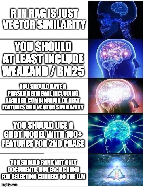
FAQ
Q: Which embedding models can I use with Vespa? A: Vespa supports a variety of embedding models. For a list of vespa provided models on Vespa Cloud, see Model hub. See also embedding reference for how to use embedders. You can also use private models (gated by authentication with Bearer token from Vespa Cloud secret store).
Q: Why don't you use ColBERT for ranking? A: We love ColBERT, and it has shown great performance. We do support ColBERT-style models in Vespa. The challenge is the added cost in memory storage, especially for large-scale applications. If you use it, we recommend consider binarizing the vectors to reduce memory usage 32x compared to float. If you want to improve the ranking quality and accept the additional cost, we encourage you to evaluate and try. Here are some resources if you want to learn more about using ColBERT with Vespa:
Q: Do I need to use an LLM with Vespa? A: No, you are free to use Vespa as a search engine. We provide the option of calling out to LLMs from within a Vespa application for reduced latency compared to sending large search results sets several times over network as well as the option to deploy Local LLMs, optionally in your own infrastructure if you prefer. See Vespa Cloud Enclave
Q: Why do we use binary vectors for the document embeddings? A: Binary vectors takes up a lot less memory and are faster to compute distances on, with only a slight reduction in quality. See blog post for details.
Q: How can you say that Vespa can scale to any data and query load? A: Vespa can scale both the stateless container nodes and content nodes of your application. See overview and elasticity for details.
Clean up
As this tutorial is running in a CI environment, we will clean up the resources created.
if os.getenv("CI", "false") == "true":
    vespa_cloud.delete()